4.2 t-tests
4.2.1 Independent samples t-test
Say we want to test whether men and women differ in the degree to which they are dominant. Let’s create a boxplot first and then check the means and the standard deviations:
ggplot(data = powercc, mapping = aes(x = gender, y = dominance)) +
  geom_boxplot()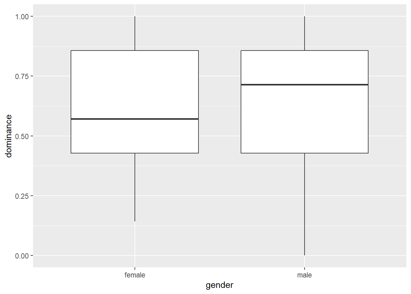
powercc %>%
  group_by(gender) %>%
  summarize(mean_dominance = mean(dominance),
            sd_dominance = sd(dominance))
## `summarise()` ungrouping output (override with `.groups` argument)## # A tibble: 2 x 3
## gender mean_dominance sd_dominance
## <chr> <dbl> <dbl>
## 1 female 0.614 0.247
## 2 male 0.646 0.296Men score slightly higher than women, but we want to know whether this difference is significant. An independent samples t-test can provide the answer (the men and the women in our experiment are the independent samples), but we need to check an assumption first: are the variances of the two independent samples equal?
install.packages("car") # for the test of equal variances, we need a package called car
library(car)
# Levene's test of equal variances.
# Low p-value means the variances are not equal.
# First argument = continuous dependent variable, second argument = categorical independent variable.
leveneTest(powercc$dominance, powercc$gender) ## Levene's Test for Homogeneity of Variance (center = median)
## Df F value Pr(>F)
## group 1 2.1915 0.141
## 141The null hypothesis of equal variances is not rejected (p = 0.14), so we can continue with a t-test that assumes equal variances:
# Test whether the means of dominance differ between genders.
# Indicate whether the test should assume equal variances or not (set var.equal = FALSE for a test that does not assume equal variances).
t.test(powercc$dominance ~ powercc$gender, var.equal = TRUE)
##
## Two Sample t-test
##
## data: powercc$dominance by powercc$gender
## t = -0.6899, df = 141, p-value = 0.4914
## alternative hypothesis: true difference in means is not equal to 0
## 95 percent confidence interval:
## -0.12179092 0.05877722
## sample estimates:
## mean in group female mean in group male
## 0.6142857 0.6457926You could report this as follows: “Men (M = 0.65, SD = 0.3) and women (M = 0.61, SD = 0.25) did not differ in the degree to which they rated themselves as dominant (t(141) = -0.69, p = 0.49).”
4.2.2 Dependent samples t-test
Say we want to test whether people are more willing to spend on conspicuous items than on inconspicuous items. Let’s check the means and the standard deviations first:
powercc %>% # no need to group! we're not splitting up our sample into subgroups
  summarize(mean_cc = mean(cc), sd_cc = sd(cc),
            mean_icc = mean(icc), sd_icc = sd(icc))
## # A tibble: 1 x 4
## mean_cc sd_cc mean_icc sd_icc
## <dbl> <dbl> <dbl> <dbl>
## 1 6.01 1.05 3.60 0.988The means are higher for conspicuous products than for inconspicuous products, but we want to know whether this difference is significant and therefore perform a dependent samples t-test (each participant rates both conspicuous and inconspicuous products, so these ratings are dependent):
t.test(powercc$cc, powercc$icc, paired = TRUE) # Test whether the means of cc and icc are different. Indicate that this is a dependent samples t-test with paired = TRUE.##
## Paired t-test
##
## data: powercc$cc and powercc$icc
## t = 25.064, df = 142, p-value < 2.2e-16
## alternative hypothesis: true difference in means is not equal to 0
## 95 percent confidence interval:
## 2.214575 2.593816
## sample estimates:
## mean of the differences
## 2.404196You could report this as follows: “People indicated they were willing to pay more (t(142) = 25.064, p < .001) for conspicuous products (M = 6.01, SD = 1.05) than for inconspicuous products (M = 3.6, SD = 0.99).”
4.2.3 One sample t-test
Say we want to test whether the average willingness to pay for the conspicuous items was significantly higher than 5 (the midpoint of the scale):
t.test(powercc$cc, mu = 5) # Indicate the variable whose mean we want to compare with a specific value (5).##
## One Sample t-test
##
## data: powercc$cc
## t = 11.499, df = 142, p-value < 2.2e-16
## alternative hypothesis: true mean is not equal to 5
## 95 percent confidence interval:
## 5.833886 6.180100
## sample estimates:
## mean of x
## 6.006993It’s indeed significantly higher than 5. You could report this as follows: “The average WTP for conspicuous products (M = 6.01, SD = 1.05) was significantly above 5 (t(142) = 11.499, p < .001).”