3.4 Linear regression
3.4.1 Simple linear regression
Say we want to predict price based on a number of room characteristics. Let’s start with a simple case where we predict price based on one predictor: overall satisfaction. Overall satisfaction is the rating that a listing gets on airbnb.com. Let’s make a scatterplot first:
ggplot(data = airbnb, mapping = aes(x = overall_satisfaction, y = price)) +
  geom_jitter() # jitter instead of points, otherwise many dots get drawn over each other
## Warning: Removed 7064 rows containing missing values (geom_point).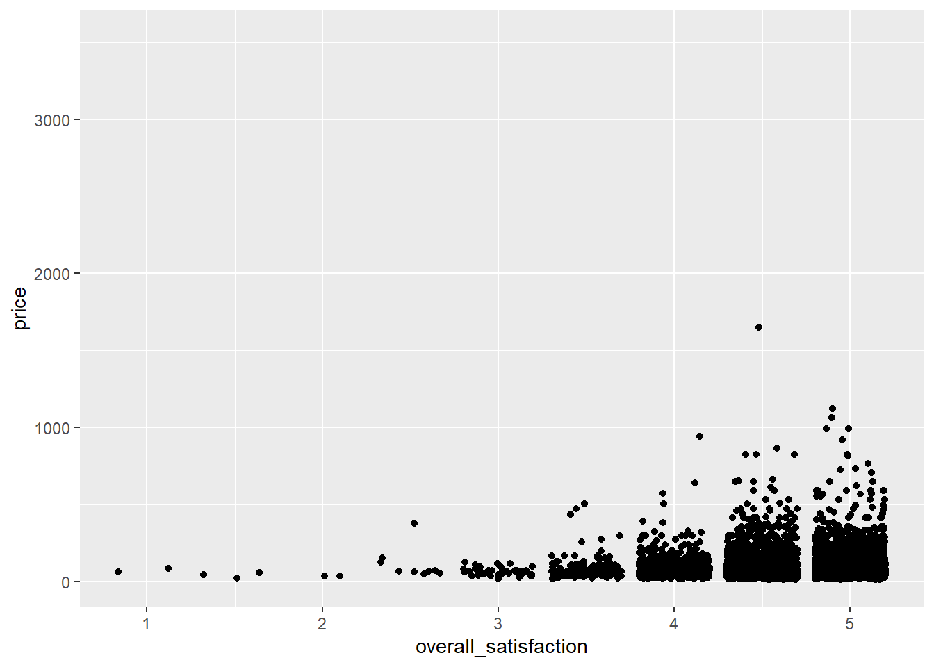
(We get an error message informing us that a number of rows were removed. These are the rows with missing values for overall_satisfaction, so there’s no need to worry about this error message. See data manipulations for why there are missing values for overall_satisfaction.)
The outliers on price reduce the informativeness of the graph, so let’s transform the price variable. Let’s also add some means to the graph, as we’ve learned here, and a regression line:
ggplot(data = airbnb, mapping = aes(x = overall_satisfaction, y = log(price, base = exp(1)))) +
  geom_jitter() + # jitter instead of points, otherwise many dots get drawn over each other
  stat_summary(fun.y=mean, colour="green", size = 4, geom="point", shape = 23, fill = "green") + # means
  stat_smooth(method = "lm", se=FALSE) # regression line
## `geom_smooth()` using formula 'y ~ x'![]()
We see that price tends to increase slightly with increased satisfaction. To test whether the relationship between price and satisfaction is indeed significant, we can perform a simple regression (simple refers to the fact that there’s only one predictor):
linearmodel <- lm(price ~ overall_satisfaction, data = airbnb) # we create a linear model. The first argument is the model which takes the form of dependent variable ~ independent variable(s). The second argument is the data we should consider.

summary(linearmodel) # ask for a summary of this linear model
##
## Call:
## lm(formula = price ~ overall_satisfaction, data = airbnb)
##
## Residuals:
## Min 1Q Median 3Q Max
## -80.51 -38.33 -15.51 14.49 1564.67
##
## Coefficients:
## Estimate Std. Error t value Pr(>|t|)
## (Intercept) 29.747 8.706 3.417 0.000636 ***
## overall_satisfaction 12.353 1.864 6.626 3.62e-11 ***
## ---
## Signif. codes: 0 '***' 0.001 '**' 0.01 '*' 0.05 '.' 0.1 ' ' 1
##
## Residual standard error: 71.47 on 10585 degrees of freedom
## (7064 observations deleted due to missingness)
## Multiple R-squared: 0.00413, Adjusted R-squared: 0.004036
## F-statistic: 43.9 on 1 and 10585 DF, p-value: 3.619e-11We see two parameters in this model:
- \(\beta_0\) or the intercept (29.75)
- \(\beta_1\) or the slope of overall satisfaction (12.35)
These parameters have the following interpretations. The intercept (\(\beta_0\)) is the estimated price for an observation with overall_satisfaction equal to zero. The slope (\(\beta_1\)) is the estimated increase in price for every increase in overall satisfaction. This determines the steepness of the fitted regression line on the graph. So for a listing that has an overall satisfaction of, for example, 3.5, the estimated price is 29.75 + 3.5 \(\times\) 12.35 = 72.98.
The slope is positive and significant. You could report this as follows: “There was a significantly positive relationship between price and overall satisfaction (\(\beta\) = 12.35, t(10585) = 6.63, p < .001).”
In the output, we also get information about the overall model. The model comes with an F value of 43.9 with 1 degree of freedom in the numerator and 10585 degrees of freedom in the denominator. This F-statistic tells us whether our model with one predictor (overall_satisfaction) predicts the dependent variable (price) better than a model without predictors (which would simply predict the average of price for every level of overall satisfaction). The degrees of freedom allow us to find the corresponding p-value (< .001) of the F-statistic (43.9). The degrees of freedom in the numerator are equal to the number of predictors in our model. The degrees of freedom in the denominator are equal to the number of observations minus the number of predictors minus one. Remember that we have 10587 observations for which we have values for both price and overall_satisfaction. The p-value is smaller than .05, so we reject the null hypothesis that our model does not predict the dependent variable better than a model without predictors. Note that in the case of simple linear regression, the p-value of the model corresponds to the p-value of the single predictor. For models with more predictors, there is no such correspondence.
Finally, also note the R-squared statistic of the model. This statistic is equal to 0.004. This statistic tells us how much of the variance in the dependent variable is explained by our predictors. The more predictors you add to a model, the higher the R-squared will be.
3.4.2 Correlations
Note that in simple linear regression, the slope of the predictor is a function of the correlation between predictor and dependent variable. We can calculate the correlation as follows:
# Make sure to include the use argument, otherwise the result will be NA due to the missing values on overall_satisfaction.
# The use argument instructs R to calculate the correlation based only on the observations for which we have data on price and on overall_satisfaction.

cor(airbnb$price, airbnb$overall_satisfaction, use = "pairwise.complete.obs")
## [1] 0.06426892We see that the correlation is positive, but very low (\(r\) = 0.064).
Squaring this correlation will get you the R-squared of a model with only that predictor (0.064 \(\times\) 0.064 = 0.004).
When dealing with multiple predictors (as in the next section), we may want to generate a correlation matrix. This is especially useful when checking for multicollinearity. Say we want the correlations between, price, overall_satisfaction, reviews, accommodates:
airbnb.corr <- airbnb %>%
  filter(!is.na(overall_satisfaction)) %>% # otherwise you'll see NA's in the result
  select(price, overall_satisfaction, reviews, accommodates)

cor(airbnb.corr) # get the correlation matrix
## price overall_satisfaction reviews accommodates
## price 1.00000000 0.06426892 -0.05827489 0.63409855
## overall_satisfaction 0.06426892 1.00000000 0.03229339 -0.04698709
## reviews -0.05827489 0.03229339 1.00000000 -0.03862767
## accommodates 0.63409855 -0.04698709 -0.03862767 1.00000000You can easily visualize this correlation matrix:
install.packages("corrplot") # install and load the corrplot package
library(corrplot)corrplot(cor(airbnb.corr), method = "number", type = "lower", bg = "grey") # put this in a nice table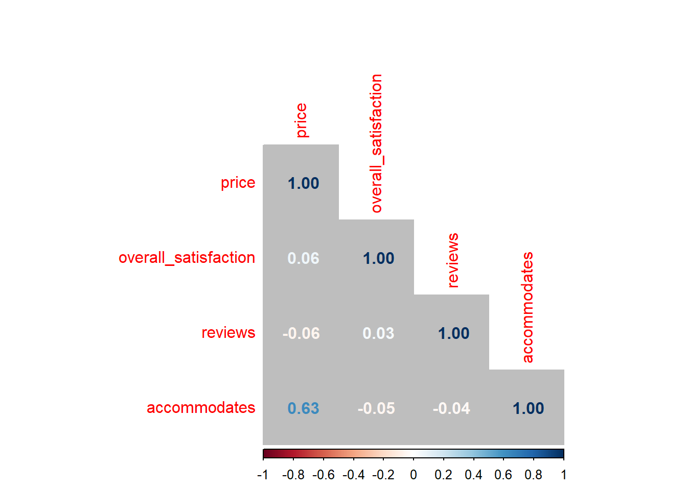
The colors of the correlations depend on their absolute values.
You can also get p-values for the correlations (p < .05 tells you the correlation differs significantly from zero):
# The command for the p-values is cor.mtest(airbnb.corr)
# But we want only the p-values, hence $p
# And we round them to five digits, hence round( , 5)

round(cor.mtest(airbnb.corr)$p, 5)
## [,1] [,2] [,3] [,4]
## [1,] 0 0.00000 0.00000 0e+00
## [2,] 0 0.00000 0.00089 0e+00
## [3,] 0 0.00089 0.00000 7e-05
## [4,] 0 0.00000 0.00007 0e+003.4.3 Multiple linear regression, without interaction
Often, we want to use more than one continuous independent variable to predict the continuous dependent variable. For example, we may want to use overall satisfaction and the number of reviews to predict the price of an Airbnb listing. The number of reviews can be seen as an indicator of how many people have stayed at a listing before. We can include both predictors (overall_satisfaction & reviews) in a model:
linearmodel <- lm(price ~ overall_satisfaction + reviews, data = airbnb)
summary(linearmodel)
##
## Call:
## lm(formula = price ~ overall_satisfaction + reviews, data = airbnb)
##
## Residuals:
## Min 1Q Median 3Q Max
## -83.18 -36.97 -16.07 13.80 1562.08
##
## Coefficients:
## Estimate Std. Error t value Pr(>|t|)
## (Intercept) 30.95504 8.69242 3.561 0.000371 ***
## overall_satisfaction 12.72777 1.86196 6.836 8.61e-12 ***
## reviews -0.10370 0.01663 -6.236 4.65e-10 ***
## ---
## Signif. codes: 0 '***' 0.001 '**' 0.01 '*' 0.05 '.' 0.1 ' ' 1
##
## Residual standard error: 71.35 on 10584 degrees of freedom
## (7064 observations deleted due to missingness)
## Multiple R-squared: 0.007776, Adjusted R-squared: 0.007589
## F-statistic: 41.48 on 2 and 10584 DF, p-value: < 2.2e-16With this model, estimated price = \(\beta_0\) + \(\beta_1\) \(\times\) overall_satisfaction + \(\beta_2\) \(\times\) reviews, where:
- \(\beta_0\) is the intercept (30.96)
- \(\beta_1\) represents the relationship between overall satisfaction and price (12.73), controlling for all other variables in our model
- \(\beta_2\) represents the relationship between reviews and price (-0.1), controlling for all other variables in our model
For a given level of reviews, the relationship between overall_satisfaction and price can be re-written as:
= [\(\beta_0\) + \(\beta_2\) \(\times\)reviews] + \(\beta_1\) \(\times\) overall_satisfaction
We see that only the intercept (\(\beta_0\) + \(\beta_2\) \(\times\)reviews) but not the slope (\(\beta_1\)) of the relationship between overall satisfaction and price depends on the number of reviews. This will change when we add an interaction between reviews and overall satisfaction (see next section).
Similarly, for a given level of overall_satisfaction, the relationship between reviews and price can be re-written as:
= [\(\beta_0\) + \(\beta_1\) \(\times\) overall_satisfaction] + \(\beta_2\) \(\times\) reviews
3.4.4 Multiple linear regression, with interaction
Often, we’re interested in interactions between predictors (e.g., overall_satisfaction & reviews). An interaction between predictors tells us that the effect of one predictor depends on the level of the other predictor:
# overall_satisfaction + reviews: the interaction is not included as a predictor
# overall_satisfaction * reviews: the interaction between the two predictors is included as a predictor

linearmodel <- lm(price ~ overall_satisfaction * reviews, data = airbnb)
summary(linearmodel)
##
## Call:
## lm(formula = price ~ overall_satisfaction * reviews, data = airbnb)
##
## Residuals:
## Min 1Q Median 3Q Max
## -82.17 -36.71 -16.08 13.47 1561.53
##
## Coefficients:
## Estimate Std. Error t value Pr(>|t|)
## (Intercept) 48.77336 10.14434 4.808 1.55e-06 ***
## overall_satisfaction 8.91437 2.17246 4.103 4.10e-05 ***
## reviews -0.99200 0.26160 -3.792 0.00015 ***
## overall_satisfaction:reviews 0.18961 0.05573 3.402 0.00067 ***
## ---
## Signif. codes: 0 '***' 0.001 '**' 0.01 '*' 0.05 '.' 0.1 ' ' 1
##
## Residual standard error: 71.31 on 10583 degrees of freedom
## (7064 observations deleted due to missingness)
## Multiple R-squared: 0.008861, Adjusted R-squared: 0.00858
## F-statistic: 31.54 on 3 and 10583 DF, p-value: < 2.2e-16With this model, estimated price = \(\beta_0\) + \(\beta_1\) \(\times\) overall_satisfaction + \(\beta_2\) \(\times\) reviews + \(\beta_3\) \(\times\) overall_satisfaction \(\times\) reviews, where:
- \(\beta_0\) is the intercept (48.77)
- \(\beta_1\) represents the relationship between overall satisfaction and price (8.91), controlling for all other variables in our model
- \(\beta_2\) represents the relationship between reviews and price (-0.99), controlling for all other variables in our model
- \(\beta_3\) is the interaction between overall satisfaction and reviews (0.19)
For a given level of reviews, the relationship between overall_satisfaction and price can be re-written as:
= [\(\beta_0\) + \(\beta_2\) \(\times\)reviews] + (\(\beta_1\) + \(\beta_3\) \(\times\) reviews) \(\times\) overall_satisfaction
We see that both the intercept (\(\beta_0\) + \(\beta_2\) \(\times\)reviews) and the slope (\(\beta_1\) + \(\beta_3\) \(\times\) reviews) of the relationship between overall satisfaction and price depend on the number of reviews. In the model without interactions, only the intercept of the relationship between overall satisfaction and price depended on the number of reviews. Because we’ve added an interaction between overall satisfaction and number of reviews to our model, the slope now also depends on the number of reviews.
Similarly, for a given level of overall_satisfaction, the relationship between reviews and price can be re-written as:
= [\(\beta_0\) + \(\beta_1\) \(\times\) overall_satisfaction] + (\(\beta_2\) + \(\beta_3\) \(\times\) overall_satisfaction) \(\times\) reviews
Here as well, we see that both the intercept and the slope of the relationship between reviews and price depend on the overall satisfaction.
As said, when the relationship between an independent variable and a dependent variable depends on the level of another independent variable, then we have an interaction between the two independent variables. For these data, the interaction is highly significant (p < .001). Let’s visualize this interaction. We focus on the relationship between overall satisfaction and price. We’ll plot this for a level of reviews that can be considered low, medium, and high:
airbnb %>%
  filter(!is.na(overall_satisfaction)) %>%
  summarize(min = min(reviews),
            Q1 = quantile(reviews, .25), # first quartile
            Q2 = quantile(reviews, .50), # second quartile or median
            Q3 = quantile(reviews, .75), # third quartile
            max = max(reviews),
            mean = mean(reviews))
## # A tibble: 1 x 6
## min Q1 Q2 Q3 max mean
## <dbl> <dbl> <dbl> <dbl> <dbl> <dbl>
## 1 3 6 13 32 708 28.5We see that 25% of listings has 6 or less reviews, 50% of listings has 13 or less reviews, and 75% of listings has 32 or less reviews.
We want three groups, however, so we could ask for different quantiles:
airbnb %>%
  filter(!is.na(overall_satisfaction)) %>%
  summarize(Q1 = quantile(reviews, .33), # low
            Q2 = quantile(reviews, .66), # medium
            max = max(reviews))          # high
## # A tibble: 1 x 3
## Q1 Q2 max
## <dbl> <dbl> <dbl>
## 1 8 23 708and make groups based on these numbers:
airbnb.reviews <- airbnb %>%
  filter(!is.na(overall_satisfaction)) %>%
  mutate(review_group = case_when(reviews <= quantile(reviews, .33) ~ "low",
                                  reviews <= quantile(reviews, .66) ~ "medium",
                                  TRUE                              ~ "high"),
         review_group = factor(review_group, levels = c("low","medium","high")))
So we tell R to make a new variable review_group that should be equal to "low" when the number of reviews is less than or equal to the 33rd percentile, "medium" when the number of reviews is less than or equal to the 66th percentile, and "high" otherwise. Afterwards, we factorize the newly created review_group variable and provide a new argument, levels, that specifies the order of the factor levels (otherwise the order would be alphabetical: high, low, medium). Let’s check whether the grouping was successful:
# check:
airbnb.reviews %>%
  group_by(review_group) %>%
  summarize(min = min(reviews), max = max(reviews))
## `summarise()` ungrouping output (override with `.groups` argument)## # A tibble: 3 x 3
## review_group min max
## <fct> <dbl> <dbl>
## 1 low 3 8
## 2 medium 9 23
## 3 high 24 708Indeed, the maximum numbers of reviews in each group correspond to the cut-off points set above. We can now ask R for a graph of the relationship between overall satisfaction and price for the three levels of review:
ggplot(data = airbnb.reviews, mapping = aes(x = overall_satisfaction, y = log(price, base = exp(1)))) + # log transform price
  facet_wrap(~ review_group) + # ask for different panels for each review group
  geom_jitter() +
  stat_smooth(method = "lm", se = FALSE)
## `geom_smooth()` using formula 'y ~ x'
We see that the relationship between overall satisfaction and price is always positive, but it is more positive for listings with many reviews than for listings with few reviews. There could be many reasons for this. Perhaps it is the case that listings with positive reviews increase their price, but only after they’ve received a certain amount of reviews.
We also see that listings with many reviews hardly ever have a satisfaction rating less than 3. This makes sense, because it is hard to keep attracting people when a listing’s rating is low. Listings with few reviews do tend to have low overall satisfaction ratings. So it seems that our predictors are correlated: the more reviews a listing has, the higher its satisfaction rating will be. This potentially presents a problem that we’ll discuss in one of the next sections on multicollinearity.
3.4.5 Assumptions
Before drawing conclusions from a regression analysis, one has to check a number of assumptions. These assumptions should be met regardless of the number of predictors in the model, but we’ll continue with the case of two predictors.
3.4.5.1 Normality of residuals
The residuals (the difference between observed and estimated values) should be normally distributed. We can visually inspect the residuals:
linearmodel <- lm(price ~ overall_satisfaction * reviews, data = airbnb)
residuals <- as_tibble(resid(linearmodel))
# ask for the residuals of the linear model with resid(linearmodel)
# and turn this in a data frame with as_tibble()

ggplot(data = residuals, mapping = aes(x = value)) +
  geom_histogram()
## `stat_bin()` using `bins = 30`. Pick better value with `binwidth`.
3.4.5.2 Homoscedasticity of residuals
The residuals (the difference between observed and estimated values) should have a constant variance. We can check this by plotting the residuals versus the predicted values:
linearmodel <- lm(price ~ overall_satisfaction * reviews, data = airbnb)

 # create a data frame (a tibble)
residuals_predicted <- tibble(residuals = resid(linearmodel), # the first variable is residuals which are the residuals of our linear model
                              predicted = predict(linearmodel)) # the second variable is predicted which are the predicted values of our linear model

ggplot(data = residuals_predicted, mapping = aes(x = predicted, y = residuals)) +
  geom_point()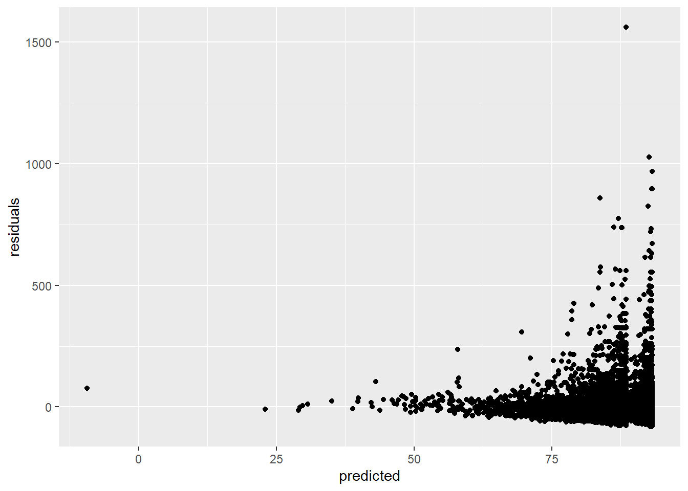
This assumption is violated, because the larger our predicted values become, the more variance we see in the residuals.
3.4.5.3 Multicollinearity
Multicollinearity exists whenever two or more of the predictors in a regression model are moderately or highly correlated (so this of course is not a problem in the case of simple regression). Let’s test the correlation between overall satisfaction and number of reviews:
# Make sure to include the use argument, otherwise the result will be NA due to the missing values on overall_satisfaction.
# The use argument instructs R to calculate the correlation based only on the observations for which we have data on price and on overall_satisfaction.

cor.test(airbnb$overall_satisfaction,airbnb$reviews, use = "pairwise.complete.obs") # test for correlation
##
## Pearson's product-moment correlation
##
## data: airbnb$overall_satisfaction and airbnb$reviews
## t = 3.3242, df = 10585, p-value = 0.0008898
## alternative hypothesis: true correlation is not equal to 0
## 95 percent confidence interval:
## 0.01325261 0.05131076
## sample estimates:
## cor
## 0.03229339Our predictors are indeed significantly correlated (p < .001), but the correlation is really low (0.03). When dealing with more than two predictors, it’s a good idea to make a correlation matrix.
The problem with multicollinearity is that it inflates the standard errors of the regression coefficients. As a result, the significance tests of these coefficients will find it harder to reject the null hypothesis. We can easily get an idea of the degree to which coefficients are inflated. To illustrate this, let’s estimate a model with predictors that are correlated: accommodates and price (\(r\) = 0.56)
linearmodel <- lm(overall_satisfaction ~  accommodates * price, data = airbnb)
summary(linearmodel)
##
## Call:
## lm(formula = overall_satisfaction ~ accommodates * price, data = airbnb)
##
## Residuals:
## Min 1Q Median 3Q Max
## -3.6494 -0.1624 -0.1105 0.3363 0.6022
##
## Coefficients:
## Estimate Std. Error t value Pr(>|t|)
## (Intercept) 4.622e+00 9.938e-03 465.031 < 2e-16 ***
## accommodates -1.640e-02 2.039e-03 -8.046 9.48e-16 ***
## price 1.356e-03 1.159e-04 11.702 < 2e-16 ***
## accommodates:price -5.423e-05 9.694e-06 -5.595 2.26e-08 ***
## ---
## Signif. codes: 0 '***' 0.001 '**' 0.01 '*' 0.05 '.' 0.1 ' ' 1
##
## Residual standard error: 0.3689 on 10583 degrees of freedom
## (7064 observations deleted due to missingness)
## Multiple R-squared: 0.0199, Adjusted R-squared: 0.01963
## F-statistic: 71.64 on 3 and 10583 DF, p-value: < 2.2e-16We see that all predictors are significant. Let’s have a look at the variance inflation factors:
library(car) # the vif function is part of the car package

vif(linearmodel)
## accommodates price accommodates:price
## 2.090206 5.359203 6.678312The VIF factors tells you the degree to which the standard errors are inflated. A rule of thumb is that VIF’s of 5 and above indicate significant inflation.