Chapter 8 Wage Analytics - Investigating the High and Low Predictors of Wages
In this assignment, I am tasked as data scientist to investigate the different factors that can predict high and low wages.
8.1 Creating the WageCategory Variable
## Warning: package 'ISLR' was built under R version 4.5.2##
## Attaching package: 'ISLR'## The following object is masked _by_ '.GlobalEnv':
##
## Wage| Name | wage |
| Number of rows | 10000 |
| Number of columns | 4 |
| _______________________ | |
| Column type frequency: | |
| factor | 2 |
| numeric | 2 |
| ________________________ | |
| Group variables | None |
Variable type: factor
| skim_variable | n_missing | complete_rate | ordered | n_unique | top_counts |
|---|---|---|---|---|---|
| default | 0 | 1 | FALSE | 2 | No: 9667, Yes: 333 |
| student | 0 | 1 | FALSE | 2 | No: 7056, Yes: 2944 |
Variable type: numeric
| skim_variable | n_missing | complete_rate | mean | sd | p0 | p25 | p50 | p75 | p100 | hist |
|---|---|---|---|---|---|---|---|---|---|---|
| balance | 0 | 1 | 835.37 | 483.71 | 0.00 | 481.73 | 823.64 | 1166.31 | 2654.32 | ▆▇▅▁▁ |
| income | 0 | 1 | 33516.98 | 13336.64 | 771.97 | 21340.46 | 34552.64 | 43807.73 | 73554.23 | ▂▇▇▅▁ |
median_wage <- median(Wage$wage, na.rm = TRUE)
Wage$WageCategory <- ifelse(Wage$wage > median_wage,
                            "High",
"Low")##
## High Low
## 1483 1517## Factor w/ 2 levels "High","Low": 2 2 1 1 2 1 1 1 1 1 ...8.2 Data Cleaning
vars_to_clean <- c("maritl", "race", "education", "region",
                   "jobclass", "health", "health_ins")

Wage[vars_to_clean] <- lapply(Wage[vars_to_clean], function(x) {
  x <- gsub("^[0-9]+\\.\\s*", "", x)
  factor(x)
})
head(Wage)
## year age maritl race education region
## 231655 2006 18 Never Married White < HS Grad Middle Atlantic
## 86582 2004 24 Never Married White College Grad Middle Atlantic
## 161300 2003 45 Married White Some College Middle Atlantic
## 155159 2003 43 Married Asian College Grad Middle Atlantic
## 11443 2005 50 Divorced White HS Grad Middle Atlantic
## 376662 2008 54 Married White College Grad Middle Atlantic
## jobclass health health_ins logwage wage WageCategory
## 231655 Industrial <=Good No 4.318063 75.04315 Low
## 86582 Information >=Very Good No 4.255273 70.47602 Low
## 161300 Industrial <=Good Yes 4.875061 130.98218 High
## 155159 Information >=Very Good Yes 5.041393 154.68529 High
## 11443 Information <=Good Yes 4.318063 75.04315 Low
## 376662 Information >=Very Good Yes 4.845098 127.11574 High8.3 Classical Statistical Tests (A)
##     High      Low
## 44.68510 40.19512##
## Welch Two Sample t-test
##
## data: age by WageCategory
## t = 10.888, df = 2855, p-value < 2.2e-16
## alternative hypothesis: true difference in means between group High and group Low is not equal to 0
## 95 percent confidence interval:
## 3.681416 5.298535
## sample estimates:
## mean in group High mean in group Low
## 44.68510 40.19512The mean for High wage earners is 44.67, and the mean for Low wage earners is 40.20. The t test shows that there is statistical difference between the two groups, which means that those who earn higher wages are more likely to be older than those who don’t.
8.3.1 Classical Statistical Tests (B)
##               Df  Sum Sq Mean Sq F value Pr(>F)
## jobclass       1  223538  223538   134.1 <2e-16 ***
## Residuals   2998 4998547    1667
## ---
## Signif. codes: 0 '***' 0.001 '**' 0.01 '*' 0.05 '.' 0.1 ' ' 1## Call:
## aov(formula = wage ~ jobclass, data = Wage)
##
## Terms:
## jobclass Residuals
## Sum of Squares 223538 4998547
## Deg. of Freedom 1 2998
##
## Residual standard error: 40.83251
## Estimated effects may be unbalancedA one-way ANOVA was conducted to examine if jobclass had an influence on wage. The ANOVA test revealed that there was a significant effect of jobclass on wage, F(1, 2998) = 134.1, p < 2e-16. It seems like different jobs lead to higher wages. Judging from this dataset, Information jobs provide higher wages than Industrial jobs.
8.3.2 Classical Statistical Tests (C)
##
##                 High  Low
##   Divorced        86  118
##   Married       1202  872
##   Never Married  169  479
##   Separated       18   37
## Widowed 8 11##
## Pearson's Chi-squared test
##
## data: tab
## X-squared = 212.51, df = 4, p-value < 2.2e-16## [1] 0.2661507X^2 = 212.51 with a p-value < 2.2x10^-16. Cramer’s V is 0.27. The chi-square analysis indicates that wage is significantly affected by marital status, and Cramer’s V result (effect size = 0.27) means that there is an association between marital status and wage.
8.4 Logistic Regression Model
## Warning: package 'caTools' was built under R version 4.5.2set.seed(123)
split <- sample.split(Wage$WageCategory, SplitRatio = 0.7)
train <- subset(Wage, split == TRUE)
test <- subset(Wage, split == FALSE)my_model <- glm(WageCategory ~ age + jobclass + education + maritl, data = train, family = binomial)
summary(my_model)##
## Call:
## glm(formula = WageCategory ~ age + jobclass + education + maritl,
## family = binomial, data = train)
##
## Coefficients:
## Estimate Std. Error z value Pr(>|z|)
## (Intercept) 3.153364 0.369325 8.538 < 2e-16 ***
## age -0.020615 0.004927 -4.185 2.86e-05 ***
## jobclassInformation -0.226817 0.104394 -2.173 0.029802 *
## educationAdvanced Degree -3.347753 0.269660 -12.415 < 2e-16 ***
## educationCollege Grad -2.386828 0.228674 -10.438 < 2e-16 ***
## educationHS Grad -0.842377 0.218824 -3.850 0.000118 ***
## educationSome College -1.543362 0.225951 -6.831 8.46e-12 ***
## maritlMarried -0.872011 0.200928 -4.340 1.43e-05 ***
## maritlNever Married 0.348751 0.236068 1.477 0.139586
## maritlSeparated -0.233811 0.424155 -0.551 0.581469
## maritlWidowed 0.335188 0.661889 0.506 0.612568
## ---
## Signif. codes: 0 '***' 0.001 '**' 0.01 '*' 0.05 '.' 0.1 ' ' 1
##
## (Dispersion parameter for binomial family taken to be 1)
##
## Null deviance: 2910.9 on 2099 degrees of freedom
## Residual deviance: 2324.4 on 2089 degrees of freedom
## AIC: 2346.4
##
## Number of Fisher Scoring iterations: 4## (Intercept) age jobclassInformation
## 23.41469156 0.97959593 0.79706683
## educationAdvanced Degree educationCollege Grad educationHS Grad
## 0.03516328 0.09192081 0.43068570
## educationSome College maritlMarried maritlNever Married
## 0.21366149 0.41810994 1.41729692
## maritlSeparated maritlWidowed
## 0.79151129 1.39820373It seems like age, education, and maritl are significant predictors for wage, specifically the High wage category. Older age is associate with a slight decrease of being in the High wage category (OR = 0.98 per year). Education seems to have the largest effect in wage (OR = 0.04). Marital status also reduces the odds of being in the High wage category (OR = 0.42). It’s interesting that jobclass shows no effect on age considering some prior data analysis.
8.5 Model Evaluation on Test Data
Prediction for High wage.
Prediction for classes.
Labeling.
## Warning: package 'caret' was built under R version 4.5.2##
## Attaching package: 'caret'## The following objects are masked from 'package:DescTools':
##
## MAE, RMSE## The following object is masked from 'package:mosaic':
##
## dotPlot## The following object is masked from 'package:purrr':
##
## lift## The following object is masked from 'package:httr':
##
## progress## Warning in confusionMatrix.default(test$pred_class, test$WageCategory,
## positive = "High"): Levels are not in the same order for reference and
## data. Refactoring data to match.## Confusion Matrix and Statistics
##
## Reference
## Prediction High Low
## High 138 330
## Low 307 125
##
## Accuracy : 0.2922
## 95% CI : (0.2627, 0.3231)
## No Information Rate : 0.5056
## P-Value [Acc > NIR] : 1.0000
##
## Kappa : -0.4149
##
## Mcnemar's Test P-Value : 0.3834
##
## Sensitivity : 0.3101
## Specificity : 0.2747
## Pos Pred Value : 0.2949
## Neg Pred Value : 0.2894
## Prevalence : 0.4944
## Detection Rate : 0.1533
## Detection Prevalence : 0.5200
## Balanced Accuracy : 0.2924
##
## 'Positive' Class : High
## Confusion Matrix.
## Warning: package 'pROC' was built under R version 4.5.2## Type 'citation("pROC")' for a citation.##
## Attaching package: 'pROC'## The following objects are masked from 'package:mosaic':
##
## cov, var## The following objects are masked from 'package:stats':
##
## cov, smooth, varroc_wage <- roc(test$WageCategory, test$pred_prob, levels = c("Low", "High"), direction = "<")
plot(roc_wage, col = "blue", main = "ROC Curve")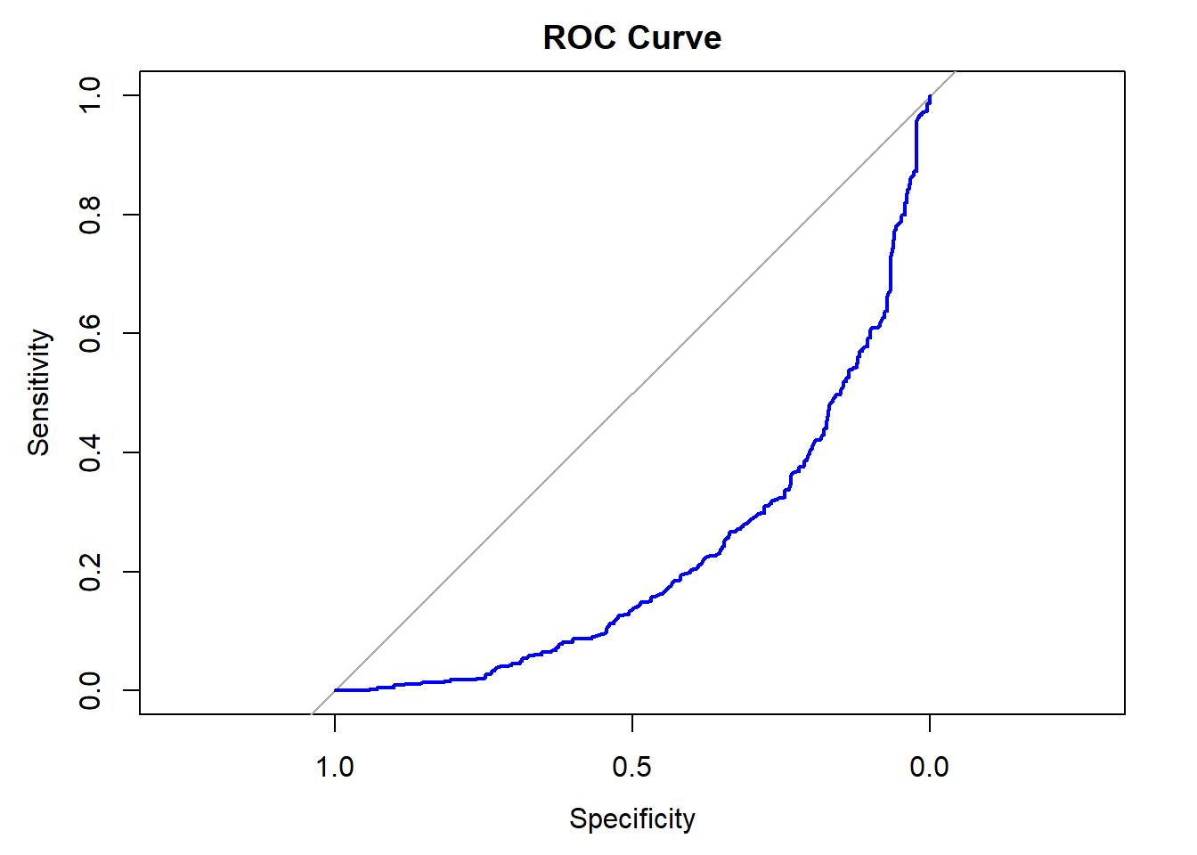 ROC Curve.
## Area under the curve: 0.2246AUC value.
8.6 Final Interpretation
The goal of this project was to investigate how different variables contribute to wage. A t-test and ANOVA revealed that wage was significantly affected by age, jobclass, and education. I saw that older ages were associated with higher earnings.
A logistic regression model was built to figure out which variables could predict the probability of being in the High wage category compared to Low wage category. Judging by the results, age, job class, education, and marital status were statistically significant in predicting wage categories. Although, sometimes depending on the analysis there were a couple of times where some predictors were non-significant.
Testing the new model on unseen showed poor predictions when it comes to Accuracy (29.2%), Sensitivity (38.3%), Specificity (31%), and ROC/AUC (0.225). It seems like this model could not distinguish between High and Low earners. Overall, age, education, job class, and marital status were significantly associated with wage. However, the logistic regression model is not reliable enough to predict wage categories with the new data. In terms of repeating the analysis, I would add years of experience, hours worked (part-time and full-time), and location (city vs suburb).