Chapter 2 R-Script

In this assignment, I learned how to pull datasets from online databases and how to clean and prepare them for data analysis.

2.1 Cleaning the data

library(httr)
library(jsonlite)
endpoint <- "https://data.cityofnewyork.us/resource/833y-fsy8.json"
resp <- httr::GET(endpoint, query = list("$limit" = 30000, "$order" = "occur_date DESC"))
shooting_data <- jsonlite::fromJSON(httr::content(resp, as = "text"), flatten = TRUE)
head(shooting_data)

##   incident_key              occur_date occur_time     boro
## 1    298699604 2024-12-31T00:00:00.000   19:16:00 BROOKLYN
## 2    298699604 2024-12-31T00:00:00.000   19:16:00 BROOKLYN
## 3    298672096 2024-12-30T00:00:00.000   16:45:00    BRONX
## 4    298672094 2024-12-30T00:00:00.000   12:15:00    BRONX
## 5    298672097 2024-12-30T00:00:00.000   18:48:00 BROOKLYN
## 6    298672096 2024-12-30T00:00:00.000   16:45:00    BRONX
##   loc_of_occur_desc precinct jurisdiction_code loc_classfctn_desc
## 1           OUTSIDE       69                 0             STREET
## 2           OUTSIDE       69                 0             STREET
## 3           OUTSIDE       47                 0             STREET
## 4           OUTSIDE       52                 0             STREET
## 5           OUTSIDE       60                 2            HOUSING
## 6           OUTSIDE       47                 0             STREET
##               location_desc statistical_murder_flag perp_age_group
## 1                    (null)                   FALSE          25-44
## 2                    (null)                   FALSE          25-44
## 3                    (null)                   FALSE         (null)
## 4                    (null)                   FALSE          45-64
## 5 MULTI DWELL - PUBLIC HOUS                   FALSE          25-44
## 6                    (null)                   FALSE         (null)
##   perp_sex perp_race vic_age_group vic_sex       vic_race x_coord_cd
## 1        M     BLACK         18-24       M          BLACK  1,015,120
## 2        M     BLACK         25-44       M          BLACK  1,015,120
## 3   (null)    (null)         18-24       M          BLACK  1,021,316
## 4        M     BLACK         25-44       M          WHITE  1,017,719
## 5        M     BLACK         45-64       M          BLACK    989,372
## 6   (null)    (null)         25-44       F WHITE HISPANIC  1,021,316
##   y_coord_cd  latitude  longitude geocoded_column.type
## 1    173,870 40.643866 -73.888761                Point
## 2    173,870 40.643866 -73.888761                Point
## 3    259,277 40.878261 -73.865964                Point
## 4    260,875 40.882661 -73.878964                Point
## 5    155,205 40.592685 -73.981557                Point
## 6    259,277 40.878261 -73.865964                Point
##   geocoded_column.coordinates
## 1         -73.88876, 40.64387
## 2         -73.88876, 40.64387
## 3         -73.86596, 40.87826
## 4         -73.87896, 40.88266
## 5         -73.98156, 40.59269
## 6         -73.86596, 40.87826

Here I gathered the NYC shooting data by using a code to bring it into R.

2.1.1 Removing NAs

library(tidyverse)
library(dplyr)
shooting_data <- shooting_data %>% filter(!is.na(geocoded_column.type))

With this code I removed NAs from geocoded_column.type.

2.1.2 Making values lowercase

shooting_data$perp_race <- tolower(shooting_data$perp_race)

I transformed uppercase letters to lowercase from the perp_race column.

2.1.3 Creating time_of_day column (Morning, Afteroon, Evening)

library(hms)
shooting_data <- shooting_data %>%
  mutate(
    occur_time = as_hms(occur_time),
    time_of_day=case_when(
      hour(occur_time)>=0 & hour(occur_time)<12 ~"morning", 
      hour(occur_time)>12 & hour(occur_time)<20 ~"afternoon", 
      TRUE ~"night"
    ))

I tried re-running the codes based on your suggestions, and it worked. I also changed the value for the for the hours just to see if it made a difference.

2.2 Insight 1

time_of_day <- shooting_data %>%
  count(time_of_day, sort = TRUE)
time_of_day

##   time_of_day     n
## 1     morning 12437
## 2       night  9340
## 3   afternoon  7870

2.3 Insight 2

vic_sex_counts <- shooting_data %>%
  count(vic_sex, sort = TRUE)
vic_sex_counts

##   vic_sex     n
## 1       M 26753
## 2       F  2882
## 3       U    12

I looked into the sex of the victims to see how crime is distributed across genders.

2.4 Tables & Graphs

library(knitr)
shooting_data <- head(shooting_data)
shooting_data

##   incident_key              occur_date occur_time     boro
## 1    298699604 2024-12-31T00:00:00.000   19:16:00 BROOKLYN
## 2    298699604 2024-12-31T00:00:00.000   19:16:00 BROOKLYN
## 3    298672096 2024-12-30T00:00:00.000   16:45:00    BRONX
## 4    298672094 2024-12-30T00:00:00.000   12:15:00    BRONX
## 5    298672097 2024-12-30T00:00:00.000   18:48:00 BROOKLYN
## 6    298672096 2024-12-30T00:00:00.000   16:45:00    BRONX
##   loc_of_occur_desc precinct jurisdiction_code loc_classfctn_desc
## 1           OUTSIDE       69                 0             STREET
## 2           OUTSIDE       69                 0             STREET
## 3           OUTSIDE       47                 0             STREET
## 4           OUTSIDE       52                 0             STREET
## 5           OUTSIDE       60                 2            HOUSING
## 6           OUTSIDE       47                 0             STREET
##               location_desc statistical_murder_flag perp_age_group
## 1                    (null)                   FALSE          25-44
## 2                    (null)                   FALSE          25-44
## 3                    (null)                   FALSE         (null)
## 4                    (null)                   FALSE          45-64
## 5 MULTI DWELL - PUBLIC HOUS                   FALSE          25-44
## 6                    (null)                   FALSE         (null)
##   perp_sex perp_race vic_age_group vic_sex       vic_race x_coord_cd
## 1        M     black         18-24       M          BLACK  1,015,120
## 2        M     black         25-44       M          BLACK  1,015,120
## 3   (null)    (null)         18-24       M          BLACK  1,021,316
## 4        M     black         25-44       M          WHITE  1,017,719
## 5        M     black         45-64       M          BLACK    989,372
## 6   (null)    (null)         25-44       F WHITE HISPANIC  1,021,316
##   y_coord_cd  latitude  longitude geocoded_column.type
## 1    173,870 40.643866 -73.888761                Point
## 2    173,870 40.643866 -73.888761                Point
## 3    259,277 40.878261 -73.865964                Point
## 4    260,875 40.882661 -73.878964                Point
## 5    155,205 40.592685 -73.981557                Point
## 6    259,277 40.878261 -73.865964                Point
##   geocoded_column.coordinates time_of_day
## 1         -73.88876, 40.64387   afternoon
## 2         -73.88876, 40.64387   afternoon
## 3         -73.86596, 40.87826   afternoon
## 4         -73.87896, 40.88266       night
## 5         -73.98156, 40.59269   afternoon
## 6         -73.86596, 40.87826   afternoon

kable(shooting_data)

incident_key	occur_date	occur_time	boro	loc_of_occur_desc	precinct	jurisdiction_code	loc_classfctn_desc	location_desc	statistical_murder_flag	perp_age_group	perp_sex	perp_race	vic_age_group	vic_sex	vic_race	x_coord_cd	y_coord_cd	latitude	longitude	geocoded_column.type	geocoded_column.coordinates	time_of_day
298699604	2024-12-31T00:00:00.000	19:16:00	BROOKLYN	OUTSIDE	69	0	STREET	(null)	FALSE	25-44	M	black	18-24	M	BLACK	1,015,120	173,870	40.643866	-73.888761	Point	-73.88876, 40.64387	afternoon
298699604	2024-12-31T00:00:00.000	19:16:00	BROOKLYN	OUTSIDE	69	0	STREET	(null)	FALSE	25-44	M	black	25-44	M	BLACK	1,015,120	173,870	40.643866	-73.888761	Point	-73.88876, 40.64387	afternoon
298672096	2024-12-30T00:00:00.000	16:45:00	BRONX	OUTSIDE	47	0	STREET	(null)	FALSE	(null)	(null)	(null)	18-24	M	BLACK	1,021,316	259,277	40.878261	-73.865964	Point	-73.86596, 40.87826	afternoon
298672094	2024-12-30T00:00:00.000	12:15:00	BRONX	OUTSIDE	52	0	STREET	(null)	FALSE	45-64	M	black	25-44	M	WHITE	1,017,719	260,875	40.882661	-73.878964	Point	-73.87896, 40.88266	night
298672097	2024-12-30T00:00:00.000	18:48:00	BROOKLYN	OUTSIDE	60	2	HOUSING	MULTI DWELL - PUBLIC HOUS	FALSE	25-44	M	black	45-64	M	BLACK	989,372	155,205	40.592685	-73.981557	Point	-73.98156, 40.59269	afternoon
298672096	2024-12-30T00:00:00.000	16:45:00	BRONX	OUTSIDE	47	0	STREET	(null)	FALSE	(null)	(null)	(null)	25-44	F	WHITE HISPANIC	1,021,316	259,277	40.878261	-73.865964	Point	-73.86596, 40.87826	afternoon

I still don’t really get what kable does… I kept getting errors for it at first, but somehow it’s working now.

2.5 Graph 1

library(ggplot2)
ggplot(shooting_data, aes(x = time_of_day, fill = time_of_day)) +
  geom_bar() +
  labs(
    title = "Shootings by Time of Day",
    x = "Time of Day",
    y = "Number of Shootings"
  ) +
  theme_minimal(base_size = 14) +
  scale_fill_brewer(palette = "Set2") +
  theme(legend.position = "none")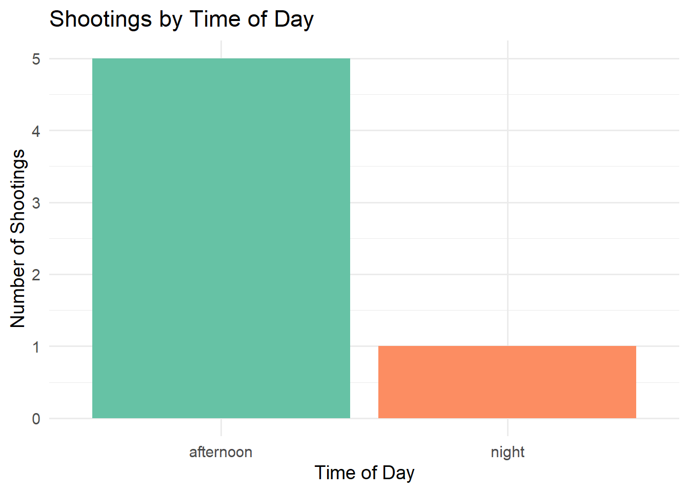

Figure 2.1: This figure shows time of day and the number of shootings.

Ahhhhhh, time_of_day is finally working!!!!!

2.6 Graph 2

library(ggplot2)
ggplot(vic_sex_counts, aes(x = vic_sex, y = n, fill = vic_sex)) +
  geom_col() +
  labs(
    title = "Victim Sex Count",
    x = "Victim Sex",
    y = "Count"
  ) +
  theme_minimal() +
  scale_fill_brewer(palette = "Pastel1") +
  theme(legend.position = "none")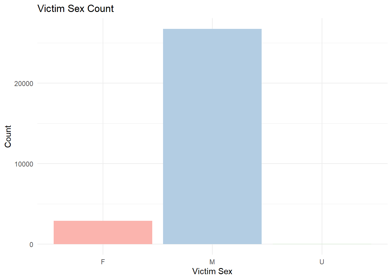

Figure 2.2: This graph shows victim counts per sex.

knitr::kable(vic_sex_counts)

vic_sex	n
M	26753
F	2882
U	12

This code allows me to have a visual representation of victims of crimes when it comes to males and females.

2.7 nrows

nrow(shooting_data)

## [1] 6

This code tells me there number of rows that remain after I cleaned up the data.

2.8 Notes

This is my second time doing this assignment. I got the chance to use the feedback and go over my lines of codes to see where I messed up. It was very helpful to do that, as I now have a better understanding when it comes to working with RMarkdown and still using R codes. I did get a few errors here and there, but this time around it was wayyyy easier to figured where they occurred in the script.