Chapter 5 NBA Analytics

Here, I investigate different teams in the NBA by looking at their stats for the regular season.

5.1 Loading and Preparing the Data

library(readxl)
team <- read_excel("data/NBA Team Total Data 2024-2025.xlsx", sheet = 18)
head(team)

## # A tibble: 6 × 30
##      Rk Player    Age     G    GS    MP    FG   FGA `FG%`  `3P` `3PA` `3P%`
##   <dbl> <chr>   <dbl> <dbl> <dbl> <dbl> <dbl> <dbl> <dbl> <dbl> <dbl> <dbl>
## 1     1 Austin…    26    73    73  2550   477  1037 0.46    200   531 0.377
## 2     2 LeBron…    40    70    70  2444   651  1270 0.513   149   396 0.376
## 3     3 Rui Ha…    26    59    57  1869   293   576 0.509   102   247 0.413
## 4     4 Gabe V…    28    72    11  1527   168   420 0.4     109   309 0.353
## 5     5 Dalton…    23    78    16  1494   257   557 0.461   128   340 0.376
## 6     6 Anthon…    31    42    42  1440   400   758 0.528    28    94 0.298
## # ℹ 18 more variables: `2P` <dbl>, `2PA` <dbl>, `2P%` <dbl>, `eFG%` <dbl>,
## #   FT <dbl>, FTA <dbl>, `FT%` <dbl>, ORB <dbl>, DRB <dbl>, TRB <dbl>,
## #   AST <dbl>, STL <dbl>, BLK <dbl>, TOV <dbl>, PF <dbl>, PTS <dbl>,
## #   `Trp-Dbl` <dbl>, Awards <chr>

library(tidyverse)
team <- team %>%
  mutate(
    Team = "Lakers",
    Won_award = ifelse(is.na(Awards), "0", "1")
  )
head(team)

## # A tibble: 6 × 32
##      Rk Player    Age     G    GS    MP    FG   FGA `FG%`  `3P` `3PA` `3P%`
##   <dbl> <chr>   <dbl> <dbl> <dbl> <dbl> <dbl> <dbl> <dbl> <dbl> <dbl> <dbl>
## 1     1 Austin…    26    73    73  2550   477  1037 0.46    200   531 0.377
## 2     2 LeBron…    40    70    70  2444   651  1270 0.513   149   396 0.376
## 3     3 Rui Ha…    26    59    57  1869   293   576 0.509   102   247 0.413
## 4     4 Gabe V…    28    72    11  1527   168   420 0.4     109   309 0.353
## 5     5 Dalton…    23    78    16  1494   257   557 0.461   128   340 0.376
## 6     6 Anthon…    31    42    42  1440   400   758 0.528    28    94 0.298
## # ℹ 20 more variables: `2P` <dbl>, `2PA` <dbl>, `2P%` <dbl>, `eFG%` <dbl>,
## #   FT <dbl>, FTA <dbl>, `FT%` <dbl>, ORB <dbl>, DRB <dbl>, TRB <dbl>,
## #   AST <dbl>, STL <dbl>, BLK <dbl>, TOV <dbl>, PF <dbl>, PTS <dbl>,
## #   `Trp-Dbl` <dbl>, Awards <chr>, Team <chr>, Won_award <chr>

library(tidyverse)
team_stat <- team %>% mutate(
  PRA=PTS+TRB+AST,
  STOCKS=STL+BLK) %>% dplyr::select("MP", "PRA", "STOCKS")
head(team_stat)

## # A tibble: 6 × 3
##      MP   PRA STOCKS
##   <dbl> <dbl>  <dbl>
## 1  2550  2225    103
## 2  2444  2831    109
## 3  1869  1153     71
## 4  1527   650     64
## 5  1494   988     32
## 6  1440  1721    144

5.2 Creating a function

all_nba <- function(x){
  team_inside <- read_excel("data/NBA Team Total Data 2024-2025.xlsx", sheet = x)
  team_inside <- team_inside %>%
  mutate(
    Team = x,
    Won_award = ifelse(is.na(Awards), "0", "1"),
    PRA=PTS+TRB+AST,
    STOCKS=STL+BLK) 
  print(team_inside)
}

library(readxl)
team_info <- excel_sheets("data/NBA Team Total Data 2024-2025.xlsx")
head(team_info)

## [1] "Nets"         "Knicks"       "Raptors"      "Philly"      
## [5] "Celtics"      "Timberwolves"

head(all_stats)

## # A tibble: 6 × 35
##      Rk Player    Age     G    GS    MP    FG   FGA `FG%`  `3P` `3PA` `3P%`
##   <dbl> <chr>   <dbl> <dbl> <dbl> <dbl> <dbl> <dbl> <dbl> <dbl> <dbl> <dbl>
## 1     1 Jalen …    24    79    22  2031   246   620 0.397   122   362 0.337
## 2     2 Keon J…    22    79    56  1925   303   779 0.389   126   401 0.314
## 3     3 Nic Cl…    25    70    62  1882   320   568 0.563     5    21 0.238
## 4     4 Camero…    28    57    57  1800   355   747 0.475   159   408 0.39 
## 5     5 Ziaire…    23    63    45  1541   214   520 0.412   103   302 0.341
## 6     6 Tyrese…    25    60    11  1315   189   465 0.406    99   282 0.351
## # ℹ 23 more variables: `2P` <dbl>, `2PA` <dbl>, `2P%` <dbl>, `eFG%` <dbl>,
## #   FT <dbl>, FTA <dbl>, `FT%` <dbl>, ORB <dbl>, DRB <dbl>, TRB <dbl>,
## #   AST <dbl>, STL <dbl>, BLK <dbl>, TOV <dbl>, PF <dbl>, PTS <dbl>,
## #   `Trp-Dbl` <dbl>, Awards <chr>, Team <chr>, Won_award <chr>, PRA <dbl>,
## #   STOCKS <dbl>, Pos <chr>

5.3 Adding Conference Information

conf <- read_excel("data/Team Conferences.xlsx")
head(conf)

## # A tibble: 6 × 2
##   Team    Conference
##   <chr>   <chr>     
## 1 Nets    East      
## 2 Knicks  East      
## 3 Raptors East      
## 4 Philly  East      
## 5 Celtics East      
## 6 Bulls   East

all_stats <- all_stats %>%
  left_join(conf, by = "Team") %>%
  mutate(
    Conference_binary = if_else(Conference == "East", 1, 0)
  )

5.4 Visual Exploration

ggplot(all_stats, aes(x = PRA, y = STOCKS, color = Conference)) +
  geom_point(alpha = 0.7) +
  labs(
    title = "PRA vs. STOCKS by Conference",
    x = "Points + Rebounds + Assists (PRA)",
    y = "Steals + Blocks (STOCKS)",
    color = "Conference"
  ) +
  theme_minimal()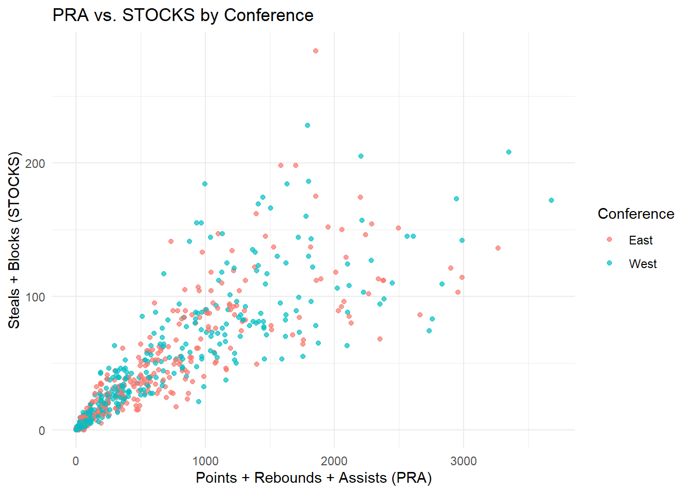

Figure 5.1: This graph shows PRA and STOCKS stats from eastern and western conference teams.

ggplot(all_stats, aes(x = PRA, fill = Conference)) +
  geom_histogram(position = "identity", alpha = 0.5, bins = 30) +
  labs(
    title = "Distribution of PRA by Conference",
    x = "PRA",
    y = "Count of Players",
    fill = "Conference"
  ) +
  theme_minimal()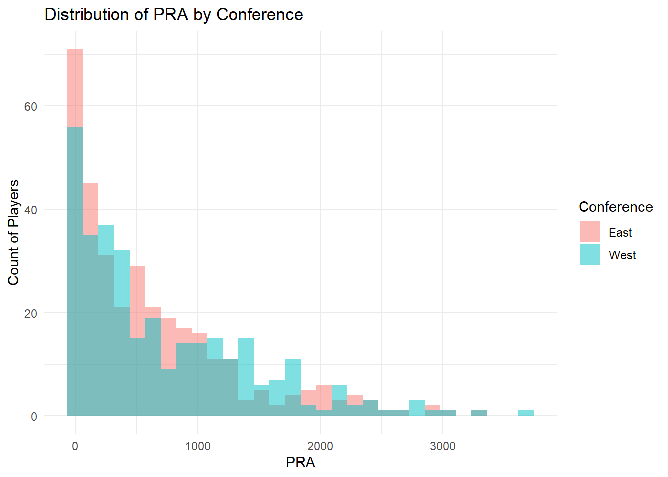

Figure 5.2: This graph shows players’ PRA by eastern and western conference.

5.5 Correlation Analysis

cor.test(all_stats$Conference_binary, all_stats$STOCKS, method = "pearson")

## 
##  Pearson's product-moment correlation
## 
## data:  x and y
## t = -2.094, df = 650, p-value = 0.03665
## alternative hypothesis: true correlation is not equal to 0
## 95 percent confidence interval:
##  -0.157650363 -0.005105577
## sample estimates:
##         cor 
## -0.08185737

cor.test(all_stats$Conference_binary, all_stats$PRA, method = "pearson")

## 
##  Pearson's product-moment correlation
## 
## data:  x and y
## t = -1.8195, df = 650, p-value = 0.0693
## alternative hypothesis: true correlation is not equal to 0
## 95 percent confidence interval:
##  -0.147164250  0.005629906
## sample estimates:
##         cor 
## -0.07118475

library(ggcorrplot)
vars <- all_stats %>% dplyr::select("Age", "PRA", "STOCKS")
cm <- round(cor(vars, use = "pairwise.complete.obs"), 3)
ggcorrplot(cm, lab = TRUE, hc.order = FALSE, type = "lower")

## Warning: `aes_string()` was deprecated in ggplot2 3.0.0.
## ℹ Please use tidy evaluation idioms with `aes()`.
## ℹ See also `vignette("ggplot2-in-packages")` for more information.
## ℹ The deprecated feature was likely used in the ggcorrplot package.
##   Please report the issue at
##   <https://github.com/kassambara/ggcorrplot/issues>.
## This warning is displayed once every 8 hours.
## Call `lifecycle::last_lifecycle_warnings()` to see where this warning was
## generated.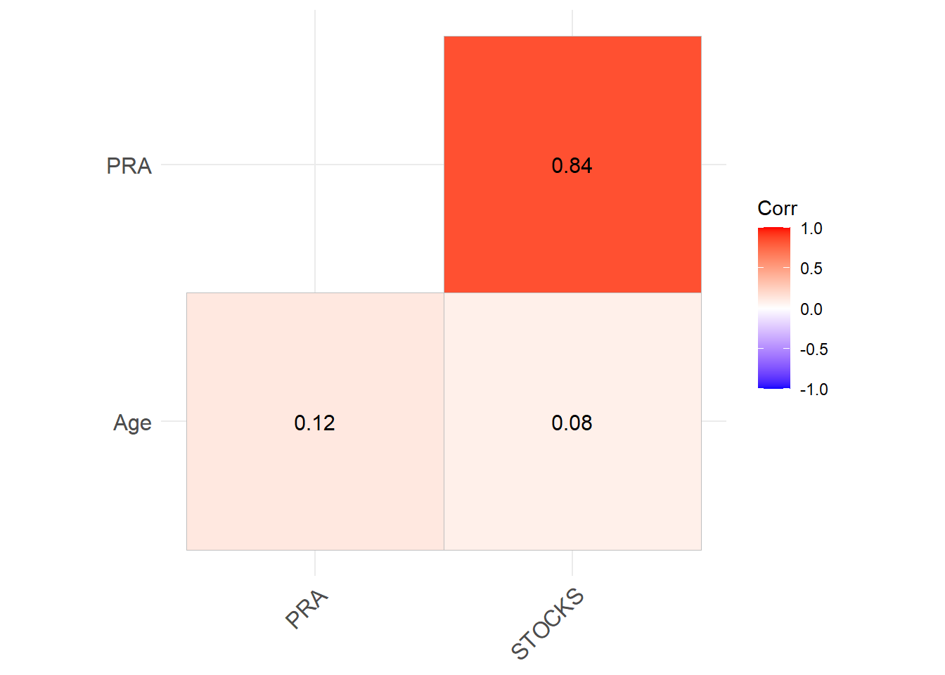

library(ppcor)

## Loading required package: MASS

## 
## Attaching package: 'MASS'

## The following object is masked from 'package:dplyr':
## 
##     select

colnames(all_stats)

##  [1] "Rk"                "Player"            "Age"              
##  [4] "G"                 "GS"                "MP"               
##  [7] "FG"                "FGA"               "FG%"              
## [10] "3P"                "3PA"               "3P%"              
## [13] "2P"                "2PA"               "2P%"              
## [16] "eFG%"              "FT"                "FTA"              
## [19] "FT%"               "ORB"               "DRB"              
## [22] "TRB"               "AST"               "STL"              
## [25] "BLK"               "TOV"               "PF"               
## [28] "PTS"               "Trp-Dbl"           "Awards"           
## [31] "Team"              "Won_award"         "PRA"              
## [34] "STOCKS"            "Pos"               "Conference"       
## [37] "Conference_binary"

pcor.test(all_stats$PRA, all_stats$STOCKS, all_stats$Age, method = "pearson")

##    estimate       p.value statistic   n gp  Method
## 1 0.8395996 3.657553e-174  39.37587 652  1 pearson

5.6 Communicate Your Findings

I have no idea what’s going on with my functions!I can’t plot nor read the graphs to come to a conclusion.! (In retrospect, this was a really fun assignment.)