12.4 Lab 13: Sentiment analysis
First we’ll need some data that contains text of any sort. We’ll work with the large set of tweets that you know from before. You can find a description here.
library(DBI)
db <- dbConnect(RSQLite::SQLite(), "./www/tweets-sentiment-db.sqlite")
dbListTables(db)
## [1] "table_tweets"dbListFields(db, "table_tweets")## [1] "target" "ids" "date" "flag" "user" "text"data <- dbGetQuery(db, "SELECT target, ids, date, user, text
FROM table_tweets
ORDER BY RANDOM()
LIMIT 10000")
dbDisconnect(db)Then we’ll need to load a couple of packages necessary to do the corresponding analyses.
# Load Packages
  library("tm")
  library("SnowballC")
  library("wordcloud")
  library("RColorBrewer")
  library("tidytext")
  library("kableExtra")
And we convert the text into the tidy text format as described in the book Text Mining with R by Julia Silge and David Robinson.
# Put text into tidytext format
text_df <- data_frame(line = 1:length(data$text), text = data$text, user = data$user, date = data$date)

  # text_df
  # Tokenization and tranform into tidy structure
text_df <- text_df %>%
unnest_tokens(word, text)
Below we produce a table the contains the most frequent words in the tweets we analyze (with stopwords).
Q: What are stopwords?
    kable(text_df %>% #   # Count words (frequency)
  anti_join(stop_words) %>%
    dplyr::count(word, sort = TRUE) %>% top_n(20),
    caption = 'Most frequent words in responses without stopwords') %>%
kable_styling(bootstrap_options = c("striped", "hover", "condensed")) %>% scroll_box(height = "400px")| word | n |
|---|---|
| day | 496 |
| quot | 478 |
| http | 437 |
| love | 411 |
| time | 369 |
| lol | 363 |
| amp | 324 |
| im | 322 |
| 2 | 266 |
| night | 258 |
| home | 241 |
| morning | 235 |
| miss | 223 |
| sad | 222 |
| 3 | 201 |
| happy | 201 |
| hope | 200 |
| 197 | |
| feel | 196 |
| haha | 196 |
And naturally we can also visualize that data in a barplot containing the most frequent words.
# library(ggplot2)
  text_df %>% # generate barplot
    dplyr::count(word, sort = TRUE) %>%
    anti_join(stop_words) %>%
    top_n(20)  %>%
    mutate(word = reorder(word, n)) %>%
    ggplot(aes(word, n)) +
    geom_col() +
    xlab(NULL) +
    coord_flip()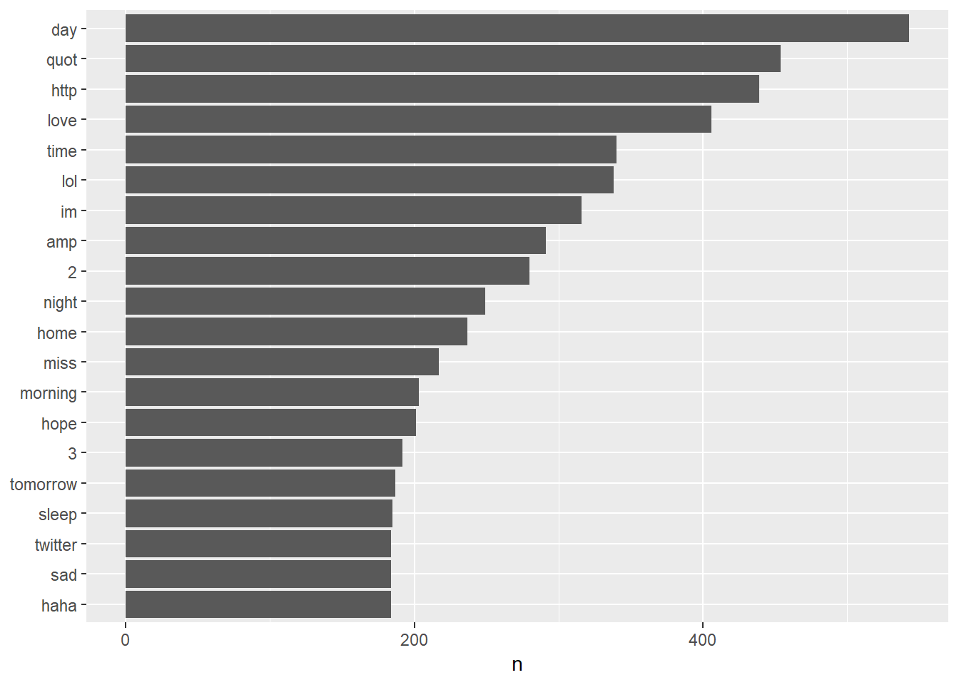
Figure 11.1: Most frequent words in open-ended answers w/o stopwords
Below we produce a table the contains the most frequent words in the tweets we analyze without stopwords.
A word cloud is another way to visualized the most frequent words in documents, e.g. tweets.
library(wordcloud)
text_df %>% # generate a wordcloud
filter(word!="crime") %>%
anti_join(stop_words) %>%
dplyr::count(word) %>%
with(wordcloud(word, n, max.words = 100))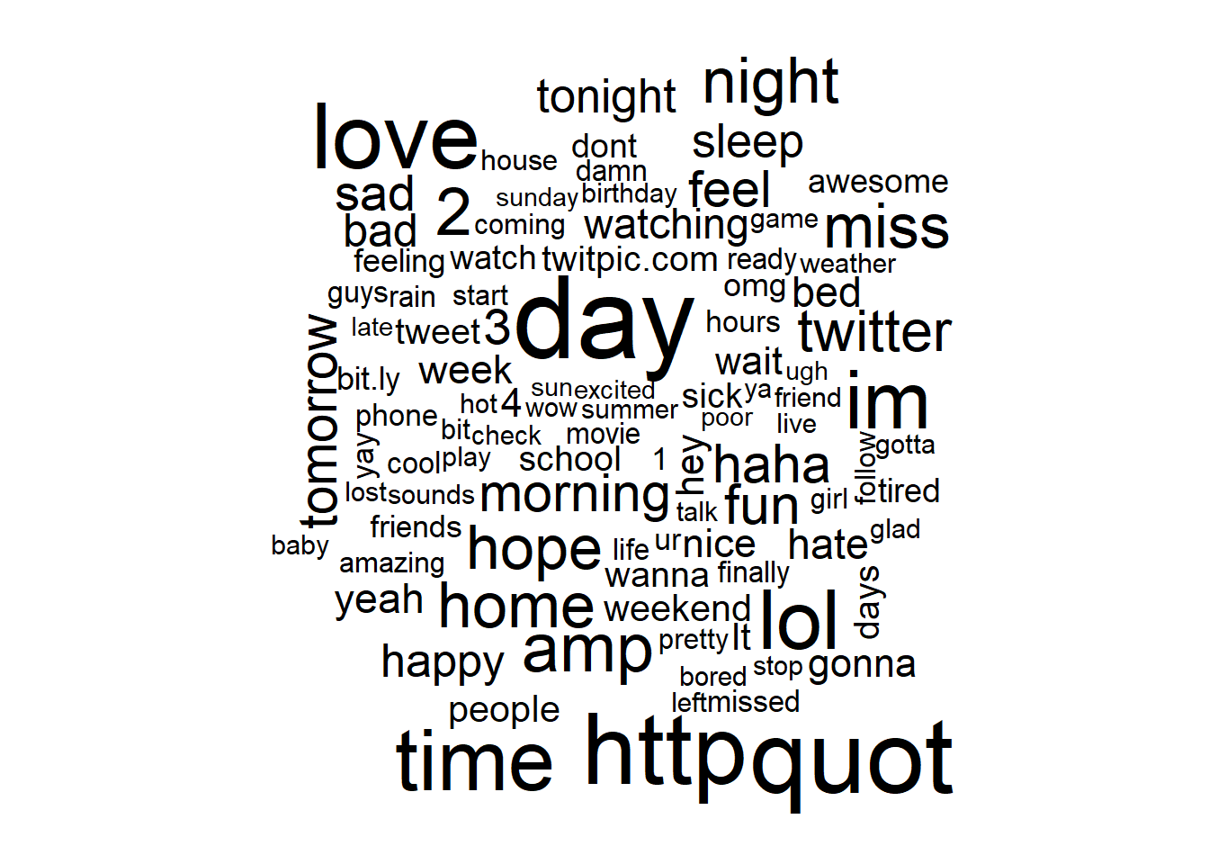
Figure 11.2: Wordcloud (w/o stopwords)
Finally, let’s try to assess the sentiment of those tweets. Wikipedia describes sentiment analysis as follows:
“Opinion mining (sometimes known as sentiment analysis or emotion AI) refers to the use of natural language processing, text analysis, computational linguistics, and biometrics to systematically identify, extract, quantify, and study affective states and subjective information. Sentiment analysis is widely applied to voice of the customer materials such as reviews and survey responses, online and social media, and healthcare materials for applications that range from marketing to customer service to clinical medicine.
Generally speaking, sentiment analysis aims to determine the attitude of a speaker, writer, or other subject with respect to some topic or the overall contextual polarity or emotional reaction to a document, interaction, or event. The attitude may be a judgment or evaluation (see appraisal theory), affective state (that is to say, the emotional state of the author or speaker), or the intended emotional communication (that is to say, the emotional effect intended by the author or interlocutor)."
Dictionary-based methods like the one we use below find the total sentiment of a document (e.g. a tweet) by adding up the individual sentiment scores for each word in the text.
Below we produce a table of the frequency of words reflecting joy that appear in the tweets. Beforehand we have to define which words reflect joy. There are different dictionaries that provide us with respective words.
# First we need to define a set of words reflecting "joy" for instance
nrcjoy <- get_sentiments("nrc") %>%
  filter(sentiment == "joy")

x <- text_df %>%
  inner_join(nrcjoy) %>%
  dplyr::count(word, sort = TRUE)

knitr::kable(x[1:10,], caption = 'Frequency of happy words') %>%
kable_styling(bootstrap_options = c("striped", "hover", "condensed"))| word | n |
|---|---|
| good | 584 |
| love | 411 |
| happy | 201 |
| hope | 200 |
| fun | 188 |
| birthday | 87 |
| feeling | 85 |
| pretty | 85 |
| luck | 78 |
| glad | 74 |
Now we’ll add sentiment scores to the original table that contains our tweets.
library(tidyr)
x <- text_df %>%
  inner_join(get_sentiments("bing")) %>% # add sentiment per word
  dplyr::count(line, index = line %/% 80, sentiment) %>% # count up positive and negative words per line/tweet
  spread(sentiment, n, fill = 0) %>% # spread out frequency of postivie/negative words in two columns
  mutate(sentiment = positive - negative) # calculate difference between number of positive and negative words

knitr::kable(x[1:10,], caption = 'Sentiment of individual statements/lines') %>%
kable_styling(bootstrap_options = c("striped", "hover", "condensed"))| line | index | negative | positive | sentiment |
|---|---|---|---|---|
| 1 | 0 | 0 | 1 | 1 |
| 2 | 0 | 1 | 0 | -1 |
| 5 | 0 | 2 | 0 | -2 |
| 8 | 0 | 0 | 1 | 1 |
| 10 | 0 | 0 | 1 | 1 |
| 11 | 0 | 0 | 1 | 1 |
| 16 | 0 | 2 | 1 | -1 |
| 18 | 0 | 0 | 1 | 1 |
| 19 | 0 | 1 | 0 | -1 |
| 20 | 0 | 1 | 0 | -1 |
# Add to sentiment estimates to dataset
data$line <- 1:nrow(data) # generate line id
data <- left_join(data, x[, c(1, 3:5)])
Then we can produce a table with the most frequent positive and negative words.
bing_word_counts <- text_df %>%
  inner_join(get_sentiments("bing")) %>%
  dplyr::count(word, sentiment, sort = TRUE) %>%
  ungroup()

knitr::kable(bing_word_counts[1:10,],
             caption = 'Most frequent positive or negative words.') %>%
kable_styling(bootstrap_options = c("striped", "hover", "condensed"))| word | sentiment | n |
|---|---|---|
| good | positive | 584 |
| like | positive | 500 |
| love | positive | 411 |
| work | positive | 398 |
| well | positive | 272 |
| miss | negative | 223 |
| sad | negative | 222 |
| happy | positive | 201 |
| great | positive | 196 |
| fun | positive | 188 |
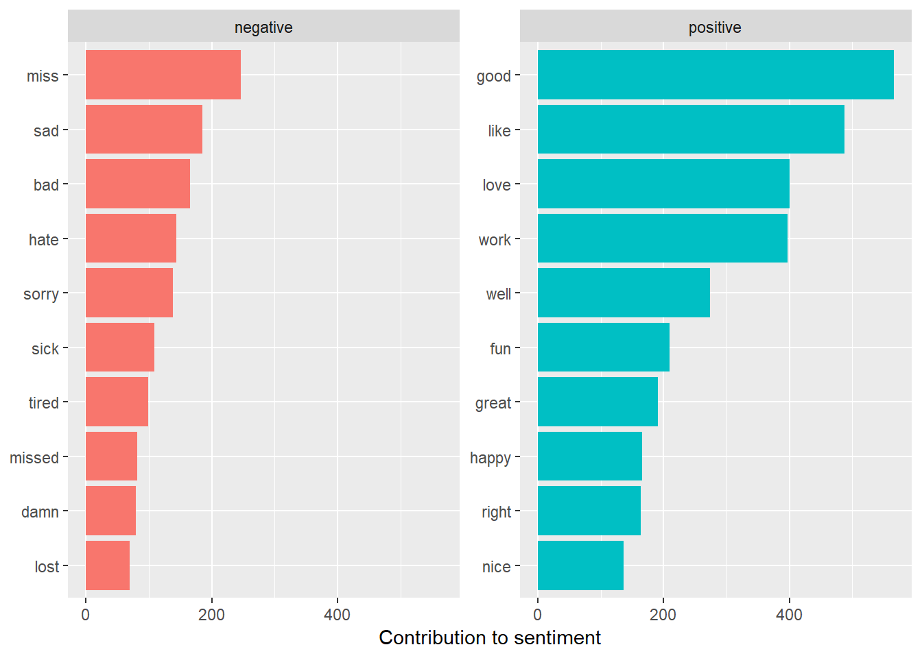
Figure 11.3: Barplot: Most common negative and positive words
Finally, a wordcloud with the postive and negative words.
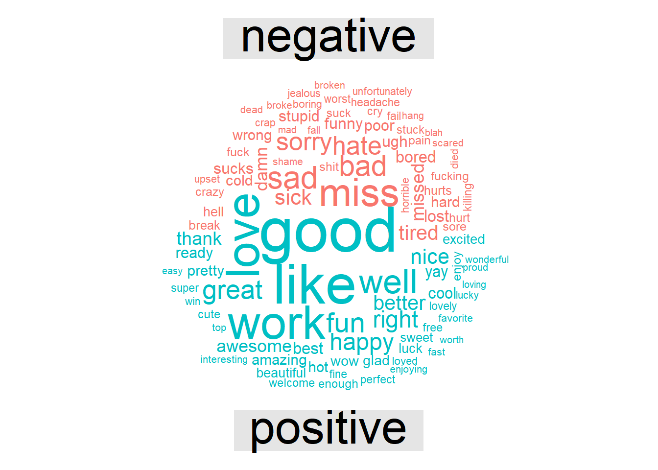
Figure 11.4: Wordcloud: Most common negative and positive words
And as a final plot a histogram of the sentiment scores across all tweets in our dataset.
library(plotly)
plot_ly(x = data$sentiment, type = "histogram") %>%
  layout(yaxis = list(title = "N"),
         xaxis = list(title = "Distribution of Sentiment Scores (Histogram)"))
Figure 11.5: Distribution of the sentiment scores: Negative/positive for negative and positive sentiment
Finally, let’s aggregate the data by user to get a ranking as to be able to compare users with regard to their overall sentiment.
library(tidyr)
data %>% group_by(user) %>% dplyr::summarise(n_tweets = n(),
                                      avg_sentiment_score = mean(sentiment, na.rm=TRUE)) %>%
arrange(desc(n_tweets), avg_sentiment_score)- Questions
- To what kind of data could we apply sentiment analysis?
- Actors? Groups? Text?
- What phenomena could we study?
- To what kind of data could we apply sentiment analysis?