4 Arboles de Decisión - Parte II
4.1 Arboles de decisión y modelos lineales
- Si la relación entre la variable dependiente y la(s) independiente se aproxima a un modelo lineal, la regresión lineal dará mejores resultados que un modelo de árbol de decisión.
- Si la relación es compleja y altamento no lineal, entonces el árbol de decisión tendrá mejores resultados de que un método clásico de regresión.
- Si se quiere construir un modelo que sea fácil de explicar, entonces un modelo de árbol de decisión será mejor que un modelo lineal.
4.2 Codigo generalizado
Existen varios algoritmos implementados ID3, CART, C4.5 C5.0, CHAID.
Es importante saber que existen variadas implementaciones (librerías) de árboles de decisión en R como por ejemplo:
rpart,tree,party,ctree, etc. Algunas se diferencias en las heurísticas utilizadas para el proceso de poda del árbol y otras manejan un componente probabilísto internamente. Un ejemplo del esquema general para implementación.
> library(rpart)
> x <- cbind(x_train,y_train)
# grow tree
> fit <- rpart(y_train ~ ., data = x,method="class")
> summary(fit)
#Predict Output
> predicted= predict(fit,x_test)
4.3 Ejemplo de Arbol de Decisión + prepruning
Entrenamiento y visualización de árboles de decisión.
- Paso 1: Importar los datos
- Paso 2: Limpiar los datos
- Paso 3: Crear los conjuntos de entranamieto y test
- Paso 4: Construir el modelo
- Paso 5: Hacer la predicción
- Paso 6: Medir el rendimiento del modelo
- Paso 7: Ajustar los hyper-parámetros
4.3.1 Importar los datos
El propósito del siguiente conjunto de datos titanic es predecir que personas son más propensas a sobrevivir la colisión con el iceberg. El conjunto de datos contiene 13 variables y 1309 observaciones. Finalmente, este se encuentra ordenado por la variable X.
set.seed(678)
path <- 'https://raw.githubusercontent.com/thomaspernet/data_csv_r/master/data/titanic_csv.csv'
titanic <-read.csv(path)
str(titanic)
## 'data.frame': 1309 obs. of 13 variables:
## $ X : int 1 2 3 4 5 6 7 8 9 10 ...
## $ pclass : int 1 1 1 1 1 1 1 1 1 1 ...
## $ survived : int 1 1 0 0 0 1 1 0 1 0 ...
## $ name : Factor w/ 1307 levels "Abbing, Mr. Anthony",..: 22 24 25 26 27 31 46 47 51 55 ...
## $ sex : Factor w/ 2 levels "female","male": 1 2 1 2 1 2 1 2 1 2 ...
## $ age : num 29 0.917 2 30 25 ...
## $ sibsp : int 0 1 1 1 1 0 1 0 2 0 ...
## $ parch : int 0 2 2 2 2 0 0 0 0 0 ...
## $ ticket : Factor w/ 929 levels "110152","110413",..: 188 50 50 50 50 125 93 16 77 826 ...
## $ fare : num 211 152 152 152 152 ...
## $ cabin : Factor w/ 187 levels "","A10","A11",..: 45 81 81 81 81 151 147 17 63 1 ...
## $ embarked : Factor w/ 4 levels "","C","Q","S": 4 4 4 4 4 4 4 4 4 2 ...
## $ home.dest: Factor w/ 370 levels "","?Havana, Cuba",..: 310 232 232 232 232 238 163 25 23 230 ...head(titanic)## X pclass survived name sex
## 1 1 1 1 Allen, Miss. Elisabeth Walton female
## 2 2 1 1 Allison, Master. Hudson Trevor male
## 3 3 1 0 Allison, Miss. Helen Loraine female
## 4 4 1 0 Allison, Mr. Hudson Joshua Creighton male
## 5 5 1 0 Allison, Mrs. Hudson J C (Bessie Waldo Daniels) female
## 6 6 1 1 Anderson, Mr. Harry male
## age sibsp parch ticket fare cabin embarked
## 1 29.0000 0 0 24160 211.3375 B5 S
## 2 0.9167 1 2 113781 151.5500 C22 C26 S
## 3 2.0000 1 2 113781 151.5500 C22 C26 S
## 4 30.0000 1 2 113781 151.5500 C22 C26 S
## 5 25.0000 1 2 113781 151.5500 C22 C26 S
## 6 48.0000 0 0 19952 26.5500 E12 S
## home.dest
## 1 St Louis, MO
## 2 Montreal, PQ / Chesterville, ON
## 3 Montreal, PQ / Chesterville, ON
## 4 Montreal, PQ / Chesterville, ON
## 5 Montreal, PQ / Chesterville, ON
## 6 New York, NYtail(titanic)## X pclass survived name sex age sibsp
## 1304 1304 3 0 Yousseff, Mr. Gerious male NA 0
## 1305 1305 3 0 Zabour, Miss. Hileni female 14.5 1
## 1306 1306 3 0 Zabour, Miss. Thamine female NA 1
## 1307 1307 3 0 Zakarian, Mr. Mapriededer male 26.5 0
## 1308 1308 3 0 Zakarian, Mr. Ortin male 27.0 0
## 1309 1309 3 0 Zimmerman, Mr. Leo male 29.0 0
## parch ticket fare cabin embarked home.dest
## 1304 0 2627 14.4583 C
## 1305 0 2665 14.4542 C
## 1306 0 2665 14.4542 C
## 1307 0 2656 7.2250 C
## 1308 0 2670 7.2250 C
## 1309 0 315082 7.8750 SLos datos no están ordenados aleatoriamente sino secuencialmente de acuerdo a la variable categórica de interés. Esto es un problema importante y se debe corregir antes de dividir los datos en entrenamiento y test. Para desordenar la lista de observaciones, se puede usar la función sample().
shuffle_index <- sample(1:nrow(titanic))
head(shuffle_index)
## [1] 288 874 1078 633 887 992Ahora se usa estos índices para generar un ordenamiento aleatorio del conjunto de datos.
titanic <- titanic[shuffle_index, ]
head(titanic)
## X pclass survived
## 288 288 1 0
## 874 874 3 0
## 1078 1078 3 1
## 633 633 3 0
## 887 887 3 1
## 992 992 3 1
## name sex age
## 288 Sutton, Mr. Frederick male 61
## 874 Humblen, Mr. Adolf Mathias Nicolai Olsen male 42
## 1078 O'Driscoll, Miss. Bridget female NA
## 633 Andersson, Mrs. Anders Johan (Alfrida Konstantia Brogren) female 39
## 887 Jermyn, Miss. Annie female NA
## 992 Mamee, Mr. Hanna male NA
## sibsp parch ticket fare cabin embarked home.dest
## 288 0 0 36963 32.3208 D50 S Haddenfield, NJ
## 874 0 0 348121 7.6500 F G63 S
## 1078 0 0 14311 7.7500 Q
## 633 1 5 347082 31.2750 S Sweden Winnipeg, MN
## 887 0 0 14313 7.7500 Q
## 992 0 0 2677 7.2292 C4.3.2 Limpiar el conjunto de datos
- Existen valores NA’s, por lo tanto deben ser eliminados.
- Prescindir de variables innecesarias
- Crear-convertir variables a tipo factor de ser necesario (e.g.,
pclassysurvived)
library(dplyr)
# Drop variables
clean_titanic <- titanic %>%
select(-c(home.dest, cabin, name, ticket)) %>%
#Convert to factor level
    mutate(pclass = factor(pclass, levels = c(1, 2, 3), labels = c('Upper', 'Middle', 'Lower')),
    survived = factor(survived, levels = c(0, 1), labels = c('No', 'Yes'))) %>%
na.omit()
glimpse(clean_titanic)
## Observations: 1,045
## Variables: 9
## $ X <int> 288, 874, 633, 182, 375, 21, 560, 307, 1104, 742, 916...
## $ pclass <fctr> Upper, Lower, Lower, Upper, Middle, Upper, Middle, U...
## $ survived <fctr> No, No, No, Yes, No, Yes, Yes, No, No, No, No, No, Y...
## $ sex <fctr> male, male, female, female, male, male, female, male...
## $ age <dbl> 61.0, 42.0, 39.0, 49.0, 29.0, 37.0, 20.0, 54.0, 2.0, ...
## $ sibsp <int> 0, 0, 1, 0, 0, 1, 0, 0, 4, 0, 0, 1, 1, 0, 0, 0, 1, 1,...
## $ parch <int> 0, 0, 5, 0, 0, 1, 0, 1, 1, 0, 0, 1, 1, 0, 2, 0, 4, 0,...
## $ fare <dbl> 32.3208, 7.6500, 31.2750, 25.9292, 10.5000, 52.5542, ...
## $ embarked <fctr> S, S, S, S, S, S, S, S, S, C, S, S, S, Q, C, S, S, C...4.3.3 Dividir en conjuntos de entrenamiento y test
Antes de entrenar el modelo vamos a dividir el conjunto de datos en entrenamiento y test. La práctica común es 80-20. Crearemos una función con este propósito.
library(dplyr)
data_train <- clean_titanic %>% dplyr::sample_frac(.8)
data_test  <- dplyr::anti_join(clean_titanic, data_train, by = 'X') # se debe tener un id
data_train <- dplyr::select(data_train, -X)
data_test <- dplyr::select(data_test, -X)
head(data_train)
## pclass survived sex age sibsp parch fare embarked
## 436 Middle Yes female 7 0 2 26.2500 S
## 837 Lower No male 25 0 0 7.7417 Q
## 504 Upper Yes female 38 0 0 227.5250 C
## 754 Lower No female 26 1 0 16.1000 S
## 290 Lower No male 31 0 0 7.7750 S
## 361 Upper Yes female 64 0 2 83.1583 Cdim(data_train)## [1] 836 8dim(data_test)## [1] 209 8- Conjunto de entrenamiento = 1046 filas (instancias)
- Conjunto de test = 262 filas (instancias)
Ahora verificamos el proceso de aleatoriedad a través de las funciones prop.table() combinada con table().
prop.table(table(data_train$survived))##
## No Yes
## 0.5873206 0.4126794prop.table(table(data_test$survived))##
## No Yes
## 0.6076555 0.3923445Instalar rpart.plot
rpart.plot es una librearía que sirve para visualizaciones más elegantes de árboles de decisión. Se debe instalar a través de la consola.
install.packages("rpart.plot") 4.3.4 Construir el modelo
El comando para generar un modelo de árbol de decisión, usando la librería rpart lleva el mismo nombre.
library(rpart)
library(rpart.plot)
fit <- rpart(survived~., data = data_train, method = 'class')
rpart.plot(fit, extra = 106)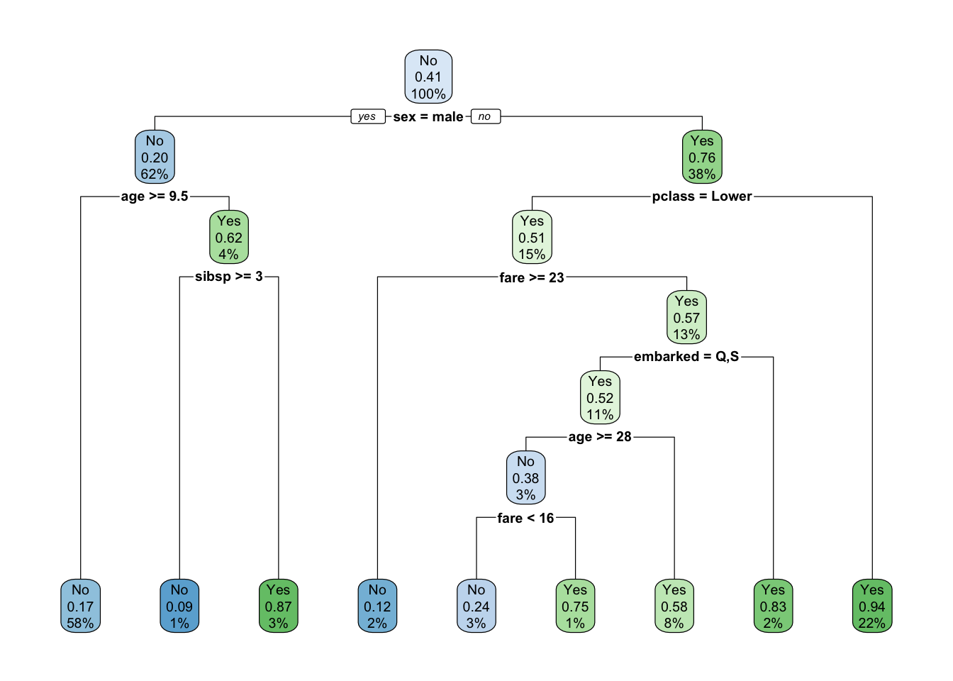
Cada nodo muestra
- La clase predecida (died o survived),
- La probabilidad predecida de survival,
- El porcentaje de observaciones en el nodo.
Ahora probemos con las opciones 1 y 9.
rpart.plot(fit, extra = 1)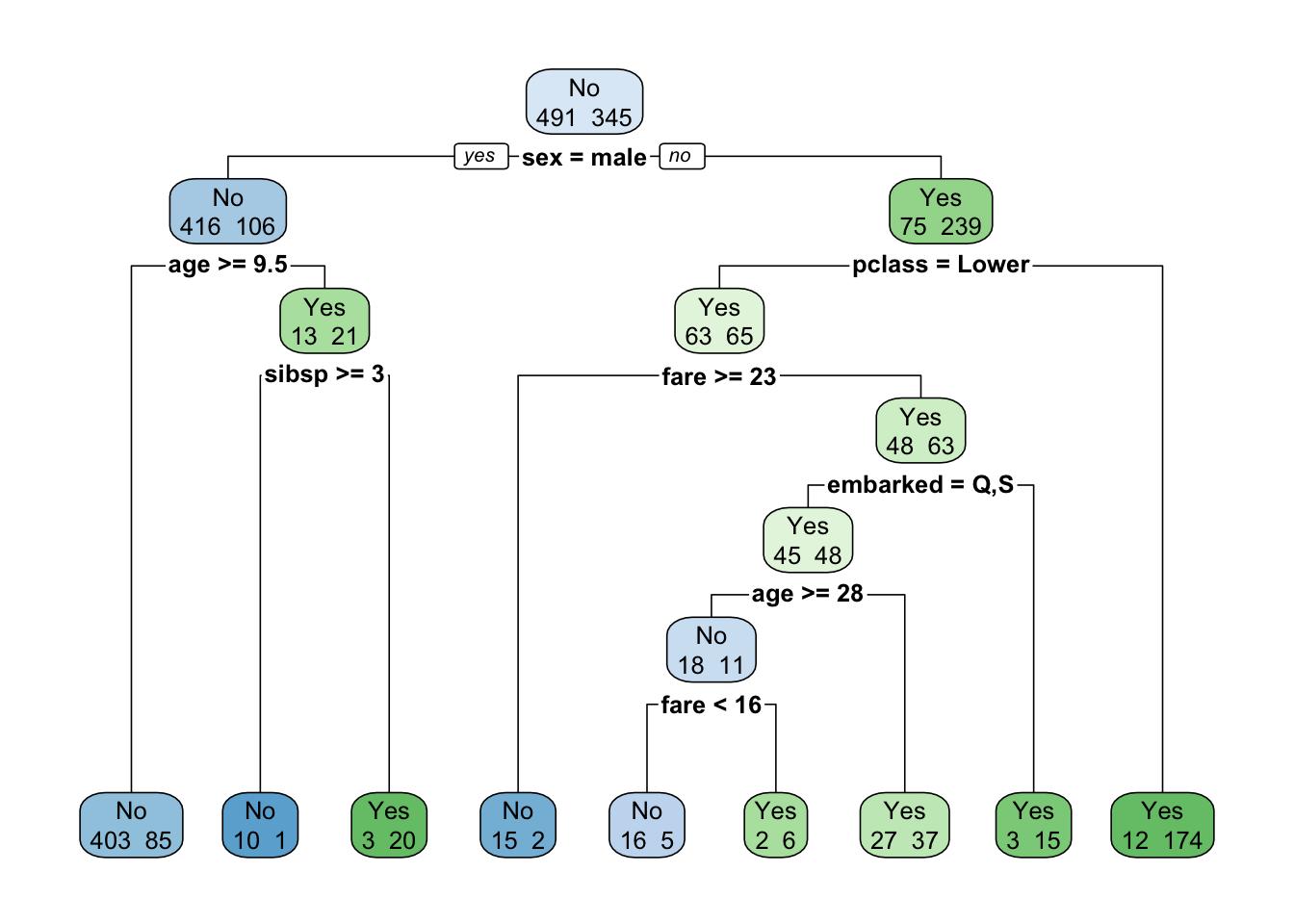
rpart.plot(fit, extra = 9)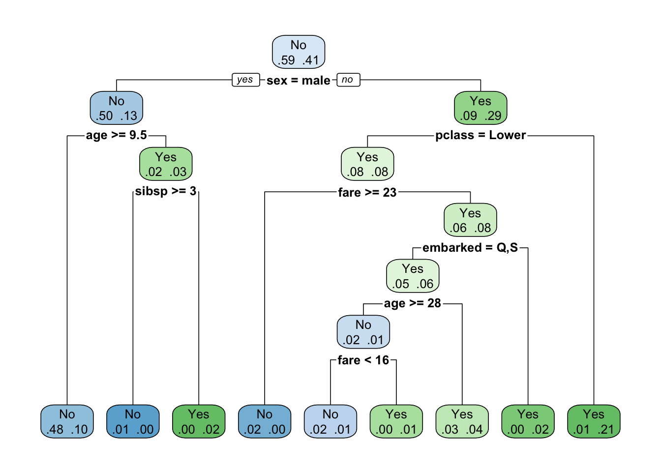
- Los árboles de decisión requieren muy poca preparación de datos. Particularmente, no requieren escalamiento de atributos o centrado.
- Por defecto,
rpart()use la medida de Gini para la división de los nodos.
4.3.5 Hacer la predicción
El modelo ha sido entrenado y ahora puede ser usado para predecir nuevas instancias en el conjunto de datos de test. Para esto se usa la función predict().
#Arguments:
#- fitted_model: This is the object stored after model estimation.
#- df: Data frame used to make the prediction
#- type: Type of prediction
#    - 'class': for classification
#    - 'prob': to compute the probability of each class
#    - 'vector': Predict the mean response at the node level

predict_unseen <-predict(fit, data_test, type = 'class')
Contabilizar la coincidencia entre las observaciones de test y los valores predecidos (matriz de confusión).
table_mat <- table(data_test$survived, predict_unseen)
table_mat
## predict_unseen
## No Yes
## No 113 14
## Yes 26 564.3.6 Medir el rendimiento del modelo
- A partir de la matriz de confusión es posible calcular un medida de rendimiento del modelo.
- La matriz de confusión es utilizada en casos de clasificación.
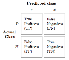
Accuracy test a partir de la matriz de confusión o tabla de contingencia
Accuracy = TP + TN / (TP + TN + FP + FN)
Proporción de las instancias predecidas correctamente TP and TN sobre la suma total de elementos evaluados.
accuracy_Test <- sum(diag(table_mat)) / sum(table_mat)
print(paste('Accuracy for test', accuracy_Test))
## [1] "Accuracy for test 0.808612440191388"4.3.7 Ajustar los hyper-parámetros
Para incluir restricciones definidas por el usuario respecto a cómo elaborar el árbol de decisión se puede utilizar el comando rpart.control() de la librería rpart.
#rpart.control(minsplit = 20, minbucket = round(minsplit/3), maxdepth = 30)
#Arguments:
#-minsplit: Set the minimum number of observations in the node before the algorithm perform a split
#-minbucket:  Set the minimum number of observations in the final node i.e. the leaf
#-maxdepth: Set the maximum depth of any node of the final tree. The root node is treated a depth 0
Vamos a modificar el ejemplo anterior. Para ello vamos a constuir una función que encapsule el cáculo de la precisión del modelo.
accuracy_tune <- function(fit) {
    predict_unseen <- predict(fit, data_test, type = 'class')
    table_mat <- table(data_test$survived, predict_unseen)
    accuracy_Test <- sum(diag(table_mat)) / sum(table_mat)
    accuracy_Test
}
Ahora, vamos a ajustar los parámetros para intentar mejor el rendimiento del modelo sobre los valores por defecto. La precisión que obtuvimos previamente fue de 0.78.
control <- rpart.control(minsplit = 4,
    minbucket = round(5 / 3),
    maxdepth = 3,
    cp = 0)
tune_fit <- rpart(survived~., data = data_train, method = 'class', control = control)
accuracy_tune(tune_fit)
## [1] 0.7990431En efecto hemos mejorado ligeramente la estimación de 0.78 a 0.79. Como habíamos revisado anteriormente, lo ideal sería aplicar un proceso de validación cruzada para ajustar correctamente y encontrar así la mejor combinación.
4.4 Ejemplo de clasificación + Poda (postpruning)
Usaremos la librería rpart para nuestro ejemplo. Esta librería incopora adicionalmente a nuestra revisión teórica, el manejo de un parámetro de regularización (optimización) que permite identificar el mejor punto para una poda.
Criterio de costo de complejidad - Cost complexity criterion
Para encontrar el balance entre la profundidad y complejidad del árbol con respecto a la capacidad predictiva del modelo en datos de test, normalmente se hace crecer el árbol de decisión hasta su mayor extensión y luego se ejecuta el proceso de poda para identificar el subárbol óptimo.
Se encuentra el subárbol óptimo usando el parámetro de costo de complejidad (\(\alpha\)) que penaliza la función objetivo abajo para el número de nodos hoja en el árbol (T)
\[minimize \left( SSE+\alpha|T| \right) \]
- Para un valor dado de \(\alpha\) se encuentra el árbol podado más pequeño (número de nodos hoja) que tiene el error más bajo de penalización.
- Se evalúan múltiples moodelos a través de un espectro de \(\alpha\) y se usa validación cruzada para identificar el \(\alpha\) óptimo, y por lo tanto el subárbol óptimo.
Ejemplo basado en https://dzone.com/articles/decision-trees-and-pruning-in-r
library(rpart)
hr_data <- read.csv("data/HR.csv")

str(hr_data)
## 'data.frame': 14999 obs. of 10 variables:
## $ satisfaction_level : num 0.38 0.8 0.11 0.72 0.37 0.41 0.1 0.92 0.89 0.42 ...
## $ last_evaluation : num 0.53 0.86 0.88 0.87 0.52 0.5 0.77 0.85 1 0.53 ...
## $ number_project : int 2 5 7 5 2 2 6 5 5 2 ...
## $ average_montly_hours : int 157 262 272 223 159 153 247 259 224 142 ...
## $ time_spend_company : int 3 6 4 5 3 3 4 5 5 3 ...
## $ Work_accident : int 0 0 0 0 0 0 0 0 0 0 ...
## $ left : int 1 1 1 1 1 1 1 1 1 1 ...
## $ promotion_last_5years: int 0 0 0 0 0 0 0 0 0 0 ...
## $ sales : Factor w/ 10 levels "IT","RandD","accounting",..: 8 8 8 8 8 8 8 8 8 8 ...
## $ salary : Factor w/ 3 levels "high","low","medium": 2 3 3 2 2 2 2 2 2 2 ...sample_ind <- sample(nrow(hr_data),nrow(hr_data)*0.70)
train <- hr_data[sample_ind,]
test <- hr_data[-sample_ind,]
#Base Model
hr_base_model <- rpart(left ~ ., data = train, method = "class",
control = rpart.control(cp = 0))
summary(hr_base_model)## Call:
## rpart(formula = left ~ ., data = train, method = "class", control = rpart.control(cp = 0))
## n= 10499
##
## CP nsplit rel error xerror xstd
## 1 0.2355305466 0 1.00000000 1.00000000 0.017512341
## 2 0.1887057878 1 0.76446945 0.76446945 0.015861870
## 3 0.0761655949 3 0.38705788 0.38705788 0.011886991
## 4 0.0526527331 5 0.23472669 0.23593248 0.009461835
## 5 0.0321543408 6 0.18207395 0.18247588 0.008376808
## 6 0.0140675241 7 0.14991961 0.15032154 0.007633241
## 7 0.0120578778 8 0.13585209 0.13866559 0.007341821
## 8 0.0064308682 9 0.12379421 0.12660772 0.007025709
## 9 0.0052250804 10 0.11736334 0.12138264 0.006883595
## 10 0.0048231511 13 0.10168810 0.11736334 0.006771987
## 11 0.0032154341 14 0.09686495 0.10450161 0.006400164
## 12 0.0028135048 15 0.09364952 0.09686495 0.006167590
## 13 0.0012057878 16 0.09083601 0.09606109 0.006142544
## 14 0.0009378349 17 0.08963023 0.09646302 0.006155081
## 15 0.0004823151 20 0.08681672 0.09766881 0.006192525
## 16 0.0004019293 25 0.08440514 0.09967846 0.006254385
## 17 0.0002679528 28 0.08319936 0.09967846 0.006254385
## 18 0.0001148369 31 0.08239550 0.10369775 0.006376123
## 19 0.0000000000 38 0.08159164 0.10490354 0.006412147
##
## Variable importance
## satisfaction_level average_montly_hours number_project
## 34 18 18
## last_evaluation time_spend_company
## 17 13
##
## Node number 1: 10499 observations, complexity param=0.2355305
## predicted class=0 expected loss=0.2369749 P(node) =1
## class counts: 8011 2488
## probabilities: 0.763 0.237
## left son=2 (7569 obs) right son=3 (2930 obs)
## Primary splits:
## satisfaction_level < 0.465 to the right, improve=1071.2240, (0 missing)
## number_project < 2.5 to the right, improve= 686.2670, (0 missing)
## time_spend_company < 2.5 to the left, improve= 288.9549, (0 missing)
## average_montly_hours < 287.5 to the left, improve= 270.1633, (0 missing)
## last_evaluation < 0.575 to the right, improve= 155.4792, (0 missing)
## Surrogate splits:
## number_project < 2.5 to the right, agree=0.793, adj=0.259, (0 split)
## average_montly_hours < 275.5 to the left, agree=0.753, adj=0.113, (0 split)
## last_evaluation < 0.485 to the right, agree=0.742, adj=0.076, (0 split)
##
## Node number 2: 7569 observations, complexity param=0.07616559
## predicted class=0 expected loss=0.09644603 P(node) =0.7209258
## class counts: 6839 730
## probabilities: 0.904 0.096
## left son=4 (6198 obs) right son=5 (1371 obs)
## Primary splits:
## time_spend_company < 4.5 to the left, improve=446.74570, (0 missing)
## last_evaluation < 0.815 to the left, improve=153.15450, (0 missing)
## average_montly_hours < 216.5 to the left, improve=120.71250, (0 missing)
## number_project < 4.5 to the left, improve= 80.28063, (0 missing)
## satisfaction_level < 0.715 to the left, improve= 58.80052, (0 missing)
## Surrogate splits:
## last_evaluation < 0.995 to the left, agree=0.823, adj=0.023, (0 split)
##
## Node number 3: 2930 observations, complexity param=0.1887058
## predicted class=1 expected loss=0.4 P(node) =0.2790742
## class counts: 1172 1758
## probabilities: 0.400 0.600
## left son=6 (1708 obs) right son=7 (1222 obs)
## Primary splits:
## number_project < 2.5 to the right, improve=310.9605, (0 missing)
## satisfaction_level < 0.115 to the right, improve=250.6215, (0 missing)
## time_spend_company < 4.5 to the right, improve=236.1650, (0 missing)
## last_evaluation < 0.575 to the right, improve=130.2469, (0 missing)
## average_montly_hours < 161.5 to the right, improve=111.4102, (0 missing)
## Surrogate splits:
## satisfaction_level < 0.355 to the left, agree=0.880, adj=0.713, (0 split)
## last_evaluation < 0.575 to the right, agree=0.859, adj=0.662, (0 split)
## average_montly_hours < 161.5 to the right, agree=0.856, adj=0.655, (0 split)
## time_spend_company < 3.5 to the right, agree=0.840, adj=0.615, (0 split)
##
## Node number 4: 6198 observations, complexity param=0.003215434
## predicted class=0 expected loss=0.01565021 P(node) =0.5903419
## class counts: 6101 97
## probabilities: 0.984 0.016
## left son=8 (6190 obs) right son=9 (8 obs)
## Primary splits:
## average_montly_hours < 290.5 to the left, improve=15.5231500, (0 missing)
## number_project < 5.5 to the left, improve= 3.7322140, (0 missing)
## satisfaction_level < 0.475 to the right, improve= 1.6447890, (0 missing)
## time_spend_company < 3.5 to the left, improve= 1.4018780, (0 missing)
## sales splits as LLLRRLLLLR, improve= 0.5033744, (0 missing)
##
## Node number 5: 1371 observations, complexity param=0.07616559
## predicted class=0 expected loss=0.4617068 P(node) =0.1305839
## class counts: 738 633
## probabilities: 0.538 0.462
## left son=10 (534 obs) right son=11 (837 obs)
## Primary splits:
## last_evaluation < 0.815 to the left, improve=301.1271, (0 missing)
## average_montly_hours < 216.5 to the left, improve=263.9916, (0 missing)
## time_spend_company < 6.5 to the right, improve=175.0792, (0 missing)
## satisfaction_level < 0.715 to the left, improve=157.5197, (0 missing)
## number_project < 3.5 to the left, improve=136.2939, (0 missing)
## Surrogate splits:
## average_montly_hours < 215.5 to the left, agree=0.743, adj=0.341, (0 split)
## number_project < 3.5 to the left, agree=0.708, adj=0.251, (0 split)
## satisfaction_level < 0.715 to the left, agree=0.705, adj=0.243, (0 split)
## time_spend_company < 6.5 to the right, agree=0.682, adj=0.184, (0 split)
## Work_accident < 0.5 to the right, agree=0.648, adj=0.097, (0 split)
##
## Node number 6: 1708 observations, complexity param=0.1887058
## predicted class=0 expected loss=0.4051522 P(node) =0.1626822
## class counts: 1016 692
## probabilities: 0.595 0.405
## left son=12 (1093 obs) right son=13 (615 obs)
## Primary splits:
## satisfaction_level < 0.115 to the right, improve=680.1184, (0 missing)
## average_montly_hours < 242.5 to the left, improve=384.2062, (0 missing)
## number_project < 5.5 to the left, improve=351.9510, (0 missing)
## last_evaluation < 0.765 to the left, improve=272.1409, (0 missing)
## time_spend_company < 3.5 to the left, improve=111.0344, (0 missing)
## Surrogate splits:
## average_montly_hours < 242.5 to the left, agree=0.856, adj=0.600, (0 split)
## number_project < 5.5 to the left, agree=0.833, adj=0.535, (0 split)
## last_evaluation < 0.765 to the left, agree=0.784, adj=0.400, (0 split)
##
## Node number 7: 1222 observations, complexity param=0.03215434
## predicted class=1 expected loss=0.1276596 P(node) =0.116392
## class counts: 156 1066
## probabilities: 0.128 0.872
## left son=14 (92 obs) right son=15 (1130 obs)
## Primary splits:
## last_evaluation < 0.575 to the right, improve=129.625400, (0 missing)
## average_montly_hours < 162 to the right, improve=117.537800, (0 missing)
## satisfaction_level < 0.355 to the left, improve=105.527700, (0 missing)
## time_spend_company < 3.5 to the right, improve= 63.082060, (0 missing)
## salary splits as LRR, improve= 7.446581, (0 missing)
## Surrogate splits:
## average_montly_hours < 162 to the right, agree=0.942, adj=0.228, (0 split)
## time_spend_company < 3.5 to the right, agree=0.938, adj=0.174, (0 split)
## satisfaction_level < 0.355 to the left, agree=0.936, adj=0.152, (0 split)
##
## Node number 8: 6190 observations, complexity param=0.0002679528
## predicted class=0 expected loss=0.01437803 P(node) =0.58958
## class counts: 6101 89
## probabilities: 0.986 0.014
## left son=16 (6080 obs) right son=17 (110 obs)
## Primary splits:
## number_project < 5.5 to the left, improve=3.3329360, (0 missing)
## satisfaction_level < 0.475 to the right, improve=1.6639030, (0 missing)
## time_spend_company < 3.5 to the left, improve=1.2096960, (0 missing)
## average_montly_hours < 247.5 to the left, improve=0.4426587, (0 missing)
## sales splits as LLLRRLLRRR, improve=0.4068224, (0 missing)
##
## Node number 9: 8 observations
## predicted class=1 expected loss=0 P(node) =0.0007619773
## class counts: 0 8
## probabilities: 0.000 1.000
##
## Node number 10: 534 observations, complexity param=0.0001148369
## predicted class=0 expected loss=0.04681648 P(node) =0.05086199
## class counts: 509 25
## probabilities: 0.953 0.047
## left son=20 (344 obs) right son=21 (190 obs)
## Primary splits:
## sales splits as LLLRLRLLRR, improve=2.3943050, (0 missing)
## average_montly_hours < 272.5 to the left, improve=2.3216550, (0 missing)
## last_evaluation < 0.805 to the left, improve=1.8136130, (0 missing)
## time_spend_company < 6.5 to the right, improve=1.4818060, (0 missing)
## satisfaction_level < 0.895 to the right, improve=0.6712242, (0 missing)
## Surrogate splits:
## last_evaluation < 0.465 to the right, agree=0.657, adj=0.037, (0 split)
## average_montly_hours < 132.5 to the right, agree=0.657, adj=0.037, (0 split)
##
## Node number 11: 837 observations, complexity param=0.05265273
## predicted class=1 expected loss=0.2735962 P(node) =0.07972188
## class counts: 229 608
## probabilities: 0.274 0.726
## left son=22 (155 obs) right son=23 (682 obs)
## Primary splits:
## average_montly_hours < 216.5 to the left, improve=160.24020, (0 missing)
## time_spend_company < 6.5 to the right, improve=132.25340, (0 missing)
## satisfaction_level < 0.715 to the left, improve=105.36270, (0 missing)
## number_project < 3.5 to the left, improve= 75.46432, (0 missing)
## salary splits as LRL, improve= 17.57553, (0 missing)
## Surrogate splits:
## time_spend_company < 6.5 to the right, agree=0.861, adj=0.252, (0 split)
## satisfaction_level < 0.715 to the left, agree=0.847, adj=0.174, (0 split)
## number_project < 3.5 to the left, agree=0.843, adj=0.155, (0 split)
##
## Node number 12: 1093 observations, complexity param=0.00522508
## predicted class=0 expected loss=0.07044831 P(node) =0.1041052
## class counts: 1016 77
## probabilities: 0.930 0.070
## left son=24 (1080 obs) right son=25 (13 obs)
## Primary splits:
## number_project < 6.5 to the left, improve=22.736150, (0 missing)
## average_montly_hours < 290.5 to the left, improve=12.174900, (0 missing)
## last_evaluation < 0.995 to the left, improve= 2.908747, (0 missing)
## sales splits as LLRLLLLLLR, improve= 2.400259, (0 missing)
## time_spend_company < 5.5 to the right, improve= 1.360632, (0 missing)
##
## Node number 13: 615 observations
## predicted class=1 expected loss=0 P(node) =0.05857701
## class counts: 0 615
## probabilities: 0.000 1.000
##
## Node number 14: 92 observations, complexity param=0.0004019293
## predicted class=0 expected loss=0.06521739 P(node) =0.008762739
## class counts: 86 6
## probabilities: 0.935 0.065
## left son=28 (85 obs) right son=29 (7 obs)
## Primary splits:
## average_montly_hours < 275.5 to the left, improve=3.8829380, (0 missing)
## sales splits as LLLLLRLLLR, improve=1.6265130, (0 missing)
## time_spend_company < 3.5 to the left, improve=1.0635450, (0 missing)
## salary splits as LRL, improve=0.4209983, (0 missing)
## satisfaction_level < 0.315 to the left, improve=0.4173913, (0 missing)
##
## Node number 15: 1130 observations, complexity param=0.01205788
## predicted class=1 expected loss=0.0619469 P(node) =0.1076293
## class counts: 70 1060
## probabilities: 0.062 0.938
## left son=30 (30 obs) right son=31 (1100 obs)
## Primary splits:
## last_evaluation < 0.445 to the left, improve=54.236520, (0 missing)
## average_montly_hours < 162 to the right, improve=47.188320, (0 missing)
## satisfaction_level < 0.35 to the left, improve=37.583870, (0 missing)
## time_spend_company < 2.5 to the left, improve=24.947510, (0 missing)
## Work_accident < 0.5 to the right, improve= 1.488762, (0 missing)
##
## Node number 16: 6080 observations
## predicted class=0 expected loss=0.01217105 P(node) =0.5791028
## class counts: 6006 74
## probabilities: 0.988 0.012
##
## Node number 17: 110 observations, complexity param=0.0002679528
## predicted class=0 expected loss=0.1363636 P(node) =0.01047719
## class counts: 95 15
## probabilities: 0.864 0.136
## left son=34 (59 obs) right son=35 (51 obs)
## Primary splits:
## sales splits as RLLLRLLLRR, improve=1.8612340, (0 missing)
## last_evaluation < 0.965 to the left, improve=1.5290910, (0 missing)
## average_montly_hours < 256.5 to the left, improve=1.3476870, (0 missing)
## satisfaction_level < 0.865 to the right, improve=1.2662340, (0 missing)
## salary splits as LRR, improve=0.3645365, (0 missing)
## Surrogate splits:
## satisfaction_level < 0.755 to the left, agree=0.591, adj=0.118, (0 split)
## salary splits as RLL, agree=0.582, adj=0.098, (0 split)
## number_project < 6.5 to the left, agree=0.573, adj=0.078, (0 split)
## average_montly_hours < 214.5 to the left, agree=0.573, adj=0.078, (0 split)
## time_spend_company < 3.5 to the left, agree=0.573, adj=0.078, (0 split)
##
## Node number 20: 344 observations
## predicted class=0 expected loss=0.01162791 P(node) =0.03276503
## class counts: 340 4
## probabilities: 0.988 0.012
##
## Node number 21: 190 observations, complexity param=0.0001148369
## predicted class=0 expected loss=0.1105263 P(node) =0.01809696
## class counts: 169 21
## probabilities: 0.889 0.111
## left son=42 (174 obs) right son=43 (16 obs)
## Primary splits:
## average_montly_hours < 272.5 to the left, improve=3.735768, (0 missing)
## last_evaluation < 0.555 to the left, improve=2.341083, (0 missing)
## Work_accident < 0.5 to the right, improve=1.703218, (0 missing)
## salary splits as RLL, improve=1.271752, (0 missing)
## satisfaction_level < 0.895 to the right, improve=1.048217, (0 missing)
##
## Node number 22: 155 observations, complexity param=0.0009378349
## predicted class=0 expected loss=0.07741935 P(node) =0.01476331
## class counts: 143 12
## probabilities: 0.923 0.077
## left son=44 (110 obs) right son=45 (45 obs)
## Primary splits:
## time_spend_company < 5.5 to the right, improve=3.5378950, (0 missing)
## number_project < 2.5 to the right, improve=2.6674830, (0 missing)
## sales splits as LLLRLLLLRR, improve=1.2673900, (0 missing)
## salary splits as LRL, improve=0.9090162, (0 missing)
## last_evaluation < 0.985 to the left, improve=0.9032991, (0 missing)
## Surrogate splits:
## average_montly_hours < 130.5 to the right, agree=0.761, adj=0.178, (0 split)
## number_project < 2.5 to the right, agree=0.748, adj=0.133, (0 split)
## sales splits as LLLRLLRLLL, agree=0.729, adj=0.067, (0 split)
## last_evaluation < 0.985 to the left, agree=0.716, adj=0.022, (0 split)
##
## Node number 23: 682 observations, complexity param=0.01406752
## predicted class=1 expected loss=0.1260997 P(node) =0.06495857
## class counts: 86 596
## probabilities: 0.126 0.874
## left son=46 (35 obs) right son=47 (647 obs)
## Primary splits:
## time_spend_company < 6.5 to the right, improve=56.351040, (0 missing)
## satisfaction_level < 0.715 to the left, improve=48.654300, (0 missing)
## number_project < 3.5 to the left, improve=44.350240, (0 missing)
## promotion_last_5years < 0.5 to the right, improve=17.076870, (0 missing)
## salary splits as LRR, improve= 8.593971, (0 missing)
## Surrogate splits:
## promotion_last_5years < 0.5 to the right, agree=0.959, adj=0.200, (0 split)
## satisfaction_level < 0.975 to the right, agree=0.952, adj=0.057, (0 split)
##
## Node number 24: 1080 observations, complexity param=0.002813505
## predicted class=0 expected loss=0.05925926 P(node) =0.1028669
## class counts: 1016 64
## probabilities: 0.941 0.059
## left son=48 (1073 obs) right son=49 (7 obs)
## Primary splits:
## average_montly_hours < 290.5 to the left, improve=12.4707300, (0 missing)
## last_evaluation < 0.995 to the left, improve= 3.1002080, (0 missing)
## satisfaction_level < 0.295 to the left, improve= 1.5340500, (0 missing)
## sales splits as LRRLLLLLLR, improve= 1.3515420, (0 missing)
## time_spend_company < 5.5 to the right, improve= 0.8342854, (0 missing)
##
## Node number 25: 13 observations
## predicted class=1 expected loss=0 P(node) =0.001238213
## class counts: 0 13
## probabilities: 0.000 1.000
##
## Node number 28: 85 observations
## predicted class=0 expected loss=0.02352941 P(node) =0.008096009
## class counts: 83 2
## probabilities: 0.976 0.024
##
## Node number 29: 7 observations
## predicted class=1 expected loss=0.4285714 P(node) =0.0006667302
## class counts: 3 4
## probabilities: 0.429 0.571
##
## Node number 30: 30 observations
## predicted class=0 expected loss=0 P(node) =0.002857415
## class counts: 30 0
## probabilities: 1.000 0.000
##
## Node number 31: 1100 observations, complexity param=0.00522508
## predicted class=1 expected loss=0.03636364 P(node) =0.1047719
## class counts: 40 1060
## probabilities: 0.036 0.964
## left son=62 (21 obs) right son=63 (1079 obs)
## Primary splits:
## average_montly_hours < 162 to the right, improve=25.5952600, (0 missing)
## satisfaction_level < 0.35 to the left, improve=17.0105900, (0 missing)
## time_spend_company < 2.5 to the left, improve=16.8526000, (0 missing)
## Work_accident < 0.5 to the right, improve= 1.0677430, (0 missing)
## last_evaluation < 0.455 to the left, improve= 0.6124402, (0 missing)
## Surrogate splits:
## time_spend_company < 2.5 to the left, agree=0.985, adj=0.238, (0 split)
## satisfaction_level < 0.295 to the left, agree=0.985, adj=0.190, (0 split)
##
## Node number 34: 59 observations
## predicted class=0 expected loss=0.05084746 P(node) =0.005619583
## class counts: 56 3
## probabilities: 0.949 0.051
##
## Node number 35: 51 observations, complexity param=0.0002679528
## predicted class=0 expected loss=0.2352941 P(node) =0.004857605
## class counts: 39 12
## probabilities: 0.765 0.235
## left son=70 (43 obs) right son=71 (8 obs)
## Primary splits:
## average_montly_hours < 256.5 to the left, improve=2.8820110, (0 missing)
## satisfaction_level < 0.595 to the right, improve=1.7431850, (0 missing)
## last_evaluation < 0.45 to the left, improve=0.8983957, (0 missing)
## salary splits as LRR, improve=0.8983957, (0 missing)
## sales splits as L---R---LR, improve=0.1434174, (0 missing)
## Surrogate splits:
## number_project < 6.5 to the left, agree=0.882, adj=0.25, (0 split)
##
## Node number 42: 174 observations, complexity param=0.0001148369
## predicted class=0 expected loss=0.08045977 P(node) =0.01657301
## class counts: 160 14
## probabilities: 0.920 0.080
## left son=84 (162 obs) right son=85 (12 obs)
## Primary splits:
## salary splits as RLL, improve=1.6483610, (0 missing)
## time_spend_company < 5.5 to the right, improve=1.3049180, (0 missing)
## last_evaluation < 0.565 to the left, improve=1.1541530, (0 missing)
## average_montly_hours < 152.5 to the left, improve=0.9341183, (0 missing)
## Work_accident < 0.5 to the right, improve=0.8831264, (0 missing)
##
## Node number 43: 16 observations
## predicted class=0 expected loss=0.4375 P(node) =0.001523955
## class counts: 9 7
## probabilities: 0.562 0.437
##
## Node number 44: 110 observations
## predicted class=0 expected loss=0.009090909 P(node) =0.01047719
## class counts: 109 1
## probabilities: 0.991 0.009
##
## Node number 45: 45 observations, complexity param=0.0009378349
## predicted class=0 expected loss=0.2444444 P(node) =0.004286122
## class counts: 34 11
## probabilities: 0.756 0.244
## left son=90 (24 obs) right son=91 (21 obs)
## Primary splits:
## number_project < 3.5 to the right, improve=4.2293650, (0 missing)
## average_montly_hours < 144.5 to the left, improve=3.5851850, (0 missing)
## sales splits as LLLRLLLRRR, improve=2.1847220, (0 missing)
## salary splits as LRL, improve=1.2230130, (0 missing)
## satisfaction_level < 0.535 to the right, improve=0.5620718, (0 missing)
## Surrogate splits:
## sales splits as LLLRRRLLRL, agree=0.711, adj=0.381, (0 split)
## satisfaction_level < 0.615 to the right, agree=0.600, adj=0.143, (0 split)
## last_evaluation < 0.895 to the right, agree=0.578, adj=0.095, (0 split)
## average_montly_hours < 101.5 to the right, agree=0.578, adj=0.095, (0 split)
## salary splits as LLR, agree=0.578, adj=0.095, (0 split)
##
## Node number 46: 35 observations
## predicted class=0 expected loss=0 P(node) =0.003333651
## class counts: 35 0
## probabilities: 1.000 0.000
##
## Node number 47: 647 observations, complexity param=0.006430868
## predicted class=1 expected loss=0.07882535 P(node) =0.06162492
## class counts: 51 596
## probabilities: 0.079 0.921
## left son=94 (26 obs) right son=95 (621 obs)
## Primary splits:
## number_project < 3.5 to the left, improve=28.781440, (0 missing)
## satisfaction_level < 0.715 to the left, improve=25.916140, (0 missing)
## average_montly_hours < 277.5 to the right, improve= 8.573654, (0 missing)
## time_spend_company < 5.5 to the right, improve= 4.287677, (0 missing)
## salary splits as LRL, improve= 2.443115, (0 missing)
## Surrogate splits:
## satisfaction_level < 0.485 to the left, agree=0.964, adj=0.115, (0 split)
## average_montly_hours < 282.5 to the right, agree=0.964, adj=0.115, (0 split)
##
## Node number 48: 1073 observations, complexity param=0.0004823151
## predicted class=0 expected loss=0.05312209 P(node) =0.1022002
## class counts: 1016 57
## probabilities: 0.947 0.053
## left son=96 (1061 obs) right son=97 (12 obs)
## Primary splits:
## last_evaluation < 0.995 to the left, improve=3.2078270, (0 missing)
## satisfaction_level < 0.295 to the left, improve=0.9214371, (0 missing)
## average_montly_hours < 131.5 to the left, improve=0.8642098, (0 missing)
## sales splits as LRRLLLLLLR, improve=0.8366530, (0 missing)
## time_spend_company < 5.5 to the right, improve=0.5995069, (0 missing)
##
## Node number 49: 7 observations
## predicted class=1 expected loss=0 P(node) =0.0006667302
## class counts: 0 7
## probabilities: 0.000 1.000
##
## Node number 62: 21 observations, complexity param=0.0004019293
## predicted class=0 expected loss=0.1904762 P(node) =0.00200019
## class counts: 17 4
## probabilities: 0.810 0.190
## left son=124 (14 obs) right son=125 (7 obs)
## Primary splits:
## satisfaction_level < 0.305 to the right, improve=3.0476190, (0 missing)
## average_montly_hours < 240.5 to the left, improve=3.0476190, (0 missing)
## sales splits as R-L-L-LRLR, improve=1.3852810, (0 missing)
## time_spend_company < 3.5 to the left, improve=0.8800366, (0 missing)
## salary splits as -LR, improve=0.6428571, (0 missing)
## Surrogate splits:
## average_montly_hours < 240.5 to the left, agree=0.905, adj=0.714, (0 split)
## sales splits as L-L-L-LLLR, agree=0.762, adj=0.286, (0 split)
## last_evaluation < 0.545 to the left, agree=0.714, adj=0.143, (0 split)
##
## Node number 63: 1079 observations, complexity param=0.00522508
## predicted class=1 expected loss=0.02131603 P(node) =0.1027717
## class counts: 23 1056
## probabilities: 0.021 0.979
## left son=126 (13 obs) right son=127 (1066 obs)
## Primary splits:
## average_montly_hours < 125.5 to the left, improve=25.2070800, (0 missing)
## satisfaction_level < 0.315 to the left, improve=11.7475200, (0 missing)
## sales splits as RLRRRRRRRR, improve= 0.5342061, (0 missing)
## last_evaluation < 0.455 to the left, improve= 0.3269398, (0 missing)
## salary splits as LRR, improve= 0.3144245, (0 missing)
## Surrogate splits:
## time_spend_company < 2.5 to the left, agree=0.99, adj=0.154, (0 split)
##
## Node number 70: 43 observations
## predicted class=0 expected loss=0.1627907 P(node) =0.004095628
## class counts: 36 7
## probabilities: 0.837 0.163
##
## Node number 71: 8 observations
## predicted class=1 expected loss=0.375 P(node) =0.0007619773
## class counts: 3 5
## probabilities: 0.375 0.625
##
## Node number 84: 162 observations, complexity param=0.0001148369
## predicted class=0 expected loss=0.0617284 P(node) =0.01543004
## class counts: 152 10
## probabilities: 0.938 0.062
## left son=168 (76 obs) right son=169 (86 obs)
## Primary splits:
## last_evaluation < 0.595 to the left, improve=1.0910130, (0 missing)
## satisfaction_level < 0.715 to the left, improve=0.6754688, (0 missing)
## time_spend_company < 5.5 to the right, improve=0.5640528, (0 missing)
## average_montly_hours < 152.5 to the left, improve=0.5198181, (0 missing)
## Work_accident < 0.5 to the right, improve=0.4748338, (0 missing)
## Surrogate splits:
## average_montly_hours < 132.5 to the left, agree=0.617, adj=0.184, (0 split)
## satisfaction_level < 0.715 to the left, agree=0.605, adj=0.158, (0 split)
## number_project < 4.5 to the left, agree=0.574, adj=0.092, (0 split)
## sales splits as ---R-R--LR, agree=0.568, adj=0.079, (0 split)
## promotion_last_5years < 0.5 to the right, agree=0.549, adj=0.039, (0 split)
##
## Node number 85: 12 observations
## predicted class=0 expected loss=0.3333333 P(node) =0.001142966
## class counts: 8 4
## probabilities: 0.667 0.333
##
## Node number 90: 24 observations
## predicted class=0 expected loss=0.04166667 P(node) =0.002285932
## class counts: 23 1
## probabilities: 0.958 0.042
##
## Node number 91: 21 observations, complexity param=0.0009378349
## predicted class=0 expected loss=0.4761905 P(node) =0.00200019
## class counts: 11 10
## probabilities: 0.524 0.476
## left son=182 (12 obs) right son=183 (9 obs)
## Primary splits:
## salary splits as LRL, improve=5.3650790, (0 missing)
## average_montly_hours < 142 to the left, improve=4.7619050, (0 missing)
## sales splits as ---RLL-LRR, improve=0.7619048, (0 missing)
## satisfaction_level < 0.725 to the right, improve=0.5852814, (0 missing)
## last_evaluation < 0.895 to the right, improve=0.5723443, (0 missing)
## Surrogate splits:
## last_evaluation < 0.895 to the right, agree=0.762, adj=0.444, (0 split)
## sales splits as ---LLL-LRL, agree=0.762, adj=0.444, (0 split)
## satisfaction_level < 0.55 to the right, agree=0.667, adj=0.222, (0 split)
## average_montly_hours < 142 to the left, agree=0.667, adj=0.222, (0 split)
## number_project < 2.5 to the left, agree=0.619, adj=0.111, (0 split)
##
## Node number 94: 26 observations, complexity param=0.0004019293
## predicted class=0 expected loss=0.1923077 P(node) =0.002476426
## class counts: 21 5
## probabilities: 0.808 0.192
## left son=188 (17 obs) right son=189 (9 obs)
## Primary splits:
## satisfaction_level < 0.61 to the right, improve=3.632479, (0 missing)
## salary splits as LRL, improve=2.622378, (0 missing)
## last_evaluation < 0.935 to the right, improve=1.410256, (0 missing)
## average_montly_hours < 234 to the right, improve=1.069404, (0 missing)
## sales splits as L--LLLLLLR, improve=1.069404, (0 missing)
## Surrogate splits:
## average_montly_hours < 224 to the right, agree=0.769, adj=0.333, (0 split)
## sales splits as R--LLRLLLL, agree=0.731, adj=0.222, (0 split)
## last_evaluation < 0.935 to the right, agree=0.692, adj=0.111, (0 split)
##
## Node number 95: 621 observations, complexity param=0.004823151
## predicted class=1 expected loss=0.04830918 P(node) =0.05914849
## class counts: 30 591
## probabilities: 0.048 0.952
## left son=190 (20 obs) right son=191 (601 obs)
## Primary splits:
## satisfaction_level < 0.71 to the left, improve=23.3537000, (0 missing)
## number_project < 5.5 to the right, improve=12.9053700, (0 missing)
## sales splits as LRLRLRRRRR, improve= 1.4124590, (0 missing)
## time_spend_company < 5.5 to the right, improve= 1.2939960, (0 missing)
## salary splits as LRR, improve= 0.9955379, (0 missing)
## Surrogate splits:
## number_project < 5.5 to the right, agree=0.969, adj=0.05, (0 split)
##
## Node number 96: 1061 observations, complexity param=0.0004823151
## predicted class=0 expected loss=0.04901037 P(node) =0.1010572
## class counts: 1009 52
## probabilities: 0.951 0.049
## left son=192 (666 obs) right son=193 (395 obs)
## Primary splits:
## satisfaction_level < 0.295 to the left, improve=1.0930690, (0 missing)
## average_montly_hours < 131.5 to the left, improve=0.7305080, (0 missing)
## last_evaluation < 0.985 to the left, improve=0.6231371, (0 missing)
## sales splits as LRRLLLLRRR, improve=0.6091616, (0 missing)
## time_spend_company < 5.5 to the right, improve=0.4644825, (0 missing)
## Surrogate splits:
## time_spend_company < 3.5 to the right, agree=0.678, adj=0.134, (0 split)
## number_project < 3.5 to the right, agree=0.672, adj=0.119, (0 split)
## average_montly_hours < 138.5 to the right, agree=0.668, adj=0.109, (0 split)
## last_evaluation < 0.475 to the right, agree=0.638, adj=0.028, (0 split)
##
## Node number 97: 12 observations
## predicted class=0 expected loss=0.4166667 P(node) =0.001142966
## class counts: 7 5
## probabilities: 0.583 0.417
##
## Node number 124: 14 observations
## predicted class=0 expected loss=0 P(node) =0.00133346
## class counts: 14 0
## probabilities: 1.000 0.000
##
## Node number 125: 7 observations
## predicted class=1 expected loss=0.4285714 P(node) =0.0006667302
## class counts: 3 4
## probabilities: 0.429 0.571
##
## Node number 126: 13 observations
## predicted class=0 expected loss=0 P(node) =0.001238213
## class counts: 13 0
## probabilities: 1.000 0.000
##
## Node number 127: 1066 observations, complexity param=0.001205788
## predicted class=1 expected loss=0.009380863 P(node) =0.1015335
## class counts: 10 1056
## probabilities: 0.009 0.991
## left son=254 (9 obs) right son=255 (1057 obs)
## Primary splits:
## satisfaction_level < 0.34 to the left, improve=7.84265700, (0 missing)
## salary splits as LRR, improve=0.43675570, (0 missing)
## sales splits as RLRRRRRRRR, improve=0.15299160, (0 missing)
## last_evaluation < 0.455 to the left, improve=0.09535386, (0 missing)
## Work_accident < 0.5 to the right, improve=0.07729790, (0 missing)
## Surrogate splits:
## time_spend_company < 3.5 to the right, agree=0.994, adj=0.333, (0 split)
##
## Node number 168: 76 observations
## predicted class=0 expected loss=0 P(node) =0.007238785
## class counts: 76 0
## probabilities: 1.000 0.000
##
## Node number 169: 86 observations, complexity param=0.0001148369
## predicted class=0 expected loss=0.1162791 P(node) =0.008191256
## class counts: 76 10
## probabilities: 0.884 0.116
## left son=338 (45 obs) right son=339 (41 obs)
## Primary splits:
## time_spend_company < 5.5 to the right, improve=0.9741476, (0 missing)
## Work_accident < 0.5 to the right, improve=0.8490218, (0 missing)
## satisfaction_level < 0.71 to the left, improve=0.7369186, (0 missing)
## last_evaluation < 0.655 to the right, improve=0.6458472, (0 missing)
## average_montly_hours < 152.5 to the left, improve=0.6155951, (0 missing)
## Surrogate splits:
## average_montly_hours < 185.5 to the right, agree=0.628, adj=0.220, (0 split)
## satisfaction_level < 0.885 to the right, agree=0.581, adj=0.122, (0 split)
## last_evaluation < 0.715 to the left, agree=0.581, adj=0.122, (0 split)
## number_project < 5.5 to the left, agree=0.570, adj=0.098, (0 split)
## sales splits as ---R-L--LL, agree=0.547, adj=0.049, (0 split)
##
## Node number 182: 12 observations
## predicted class=0 expected loss=0.1666667 P(node) =0.001142966
## class counts: 10 2
## probabilities: 0.833 0.167
##
## Node number 183: 9 observations
## predicted class=1 expected loss=0.1111111 P(node) =0.0008572245
## class counts: 1 8
## probabilities: 0.111 0.889
##
## Node number 188: 17 observations
## predicted class=0 expected loss=0 P(node) =0.001619202
## class counts: 17 0
## probabilities: 1.000 0.000
##
## Node number 189: 9 observations
## predicted class=1 expected loss=0.4444444 P(node) =0.0008572245
## class counts: 4 5
## probabilities: 0.444 0.556
##
## Node number 190: 20 observations
## predicted class=0 expected loss=0.2 P(node) =0.001904943
## class counts: 16 4
## probabilities: 0.800 0.200
##
## Node number 191: 601 observations
## predicted class=1 expected loss=0.02329451 P(node) =0.05724355
## class counts: 14 587
## probabilities: 0.023 0.977
##
## Node number 192: 666 observations
## predicted class=0 expected loss=0.03153153 P(node) =0.06343461
## class counts: 645 21
## probabilities: 0.968 0.032
##
## Node number 193: 395 observations, complexity param=0.0004823151
## predicted class=0 expected loss=0.07848101 P(node) =0.03762263
## class counts: 364 31
## probabilities: 0.922 0.078
## left son=386 (344 obs) right son=387 (51 obs)
## Primary splits:
## satisfaction_level < 0.315 to the right, improve=3.6453490, (0 missing)
## last_evaluation < 0.525 to the left, improve=1.8780370, (0 missing)
## average_montly_hours < 198.5 to the left, improve=1.4977330, (0 missing)
## Work_accident < 0.5 to the right, improve=0.8886682, (0 missing)
## number_project < 5.5 to the left, improve=0.7382494, (0 missing)
##
## Node number 254: 9 observations
## predicted class=0 expected loss=0.3333333 P(node) =0.0008572245
## class counts: 6 3
## probabilities: 0.667 0.333
##
## Node number 255: 1057 observations
## predicted class=1 expected loss=0.003784295 P(node) =0.1006763
## class counts: 4 1053
## probabilities: 0.004 0.996
##
## Node number 338: 45 observations
## predicted class=0 expected loss=0.04444444 P(node) =0.004286122
## class counts: 43 2
## probabilities: 0.956 0.044
##
## Node number 339: 41 observations, complexity param=0.0001148369
## predicted class=0 expected loss=0.195122 P(node) =0.003905134
## class counts: 33 8
## probabilities: 0.805 0.195
## left son=678 (14 obs) right son=679 (27 obs)
## Primary splits:
## satisfaction_level < 0.805 to the right, improve=1.6187900, (0 missing)
## average_montly_hours < 226.5 to the left, improve=1.4336040, (0 missing)
## Work_accident < 0.5 to the right, improve=1.1447150, (0 missing)
## last_evaluation < 0.635 to the right, improve=0.8538064, (0 missing)
## salary splits as -LR, improve=0.7066202, (0 missing)
## Surrogate splits:
## promotion_last_5years < 0.5 to the right, agree=0.707, adj=0.143, (0 split)
## number_project < 5.5 to the right, agree=0.683, adj=0.071, (0 split)
## sales splits as ---L-R--RR, agree=0.683, adj=0.071, (0 split)
##
## Node number 386: 344 observations
## predicted class=0 expected loss=0.05232558 P(node) =0.03276503
## class counts: 326 18
## probabilities: 0.948 0.052
##
## Node number 387: 51 observations, complexity param=0.0004823151
## predicted class=0 expected loss=0.254902 P(node) =0.004857605
## class counts: 38 13
## probabilities: 0.745 0.255
## left son=774 (19 obs) right son=775 (32 obs)
## Primary splits:
## number_project < 3.5 to the left, improve=3.935049, (0 missing)
## sales splits as LRRLLLLRRL, improve=3.000241, (0 missing)
## satisfaction_level < 0.305 to the left, improve=1.505882, (0 missing)
## last_evaluation < 0.535 to the left, improve=1.420168, (0 missing)
## Work_accident < 0.5 to the right, improve=1.420168, (0 missing)
## Surrogate splits:
## sales splits as RRRRRRLLRR, agree=0.725, adj=0.263, (0 split)
## satisfaction_level < 0.305 to the left, agree=0.686, adj=0.158, (0 split)
## last_evaluation < 0.405 to the left, agree=0.647, adj=0.053, (0 split)
## average_montly_hours < 261.5 to the right, agree=0.647, adj=0.053, (0 split)
## time_spend_company < 5.5 to the right, agree=0.647, adj=0.053, (0 split)
##
## Node number 678: 14 observations
## predicted class=0 expected loss=0 P(node) =0.00133346
## class counts: 14 0
## probabilities: 1.000 0.000
##
## Node number 679: 27 observations, complexity param=0.0001148369
## predicted class=0 expected loss=0.2962963 P(node) =0.002571673
## class counts: 19 8
## probabilities: 0.704 0.296
## left son=1358 (19 obs) right son=1359 (8 obs)
## Primary splits:
## satisfaction_level < 0.745 to the left, improve=2.4566280, (0 missing)
## average_montly_hours < 145.5 to the left, improve=1.6592590, (0 missing)
## last_evaluation < 0.64 to the right, improve=0.9434698, (0 missing)
## salary splits as -LR, improve=0.2945534, (0 missing)
## sales splits as ---L-R--LR, improve=0.1481481, (0 missing)
## Surrogate splits:
## last_evaluation < 0.795 to the left, agree=0.778, adj=0.25, (0 split)
## average_montly_hours < 217 to the left, agree=0.778, adj=0.25, (0 split)
##
## Node number 774: 19 observations
## predicted class=0 expected loss=0 P(node) =0.001809696
## class counts: 19 0
## probabilities: 1.000 0.000
##
## Node number 775: 32 observations, complexity param=0.0004823151
## predicted class=0 expected loss=0.40625 P(node) =0.003047909
## class counts: 19 13
## probabilities: 0.594 0.406
## left son=1550 (14 obs) right son=1551 (18 obs)
## Primary splits:
## sales splits as LRRLLLRRRL, improve=5.5803570, (0 missing)
## time_spend_company < 4.5 to the left, improve=1.2041670, (0 missing)
## average_montly_hours < 157 to the right, improve=1.2041670, (0 missing)
## last_evaluation < 0.625 to the right, improve=0.9120098, (0 missing)
## salary splits as LLR, improve=0.2556818, (0 missing)
## Surrogate splits:
## last_evaluation < 0.5 to the left, agree=0.688, adj=0.286, (0 split)
## Work_accident < 0.5 to the right, agree=0.688, adj=0.286, (0 split)
## average_montly_hours < 239 to the right, agree=0.656, adj=0.214, (0 split)
## satisfaction_level < 0.305 to the left, agree=0.625, adj=0.143, (0 split)
## time_spend_company < 4.5 to the left, agree=0.625, adj=0.143, (0 split)
##
## Node number 1358: 19 observations
## predicted class=0 expected loss=0.1578947 P(node) =0.001809696
## class counts: 16 3
## probabilities: 0.842 0.158
##
## Node number 1359: 8 observations
## predicted class=1 expected loss=0.375 P(node) =0.0007619773
## class counts: 3 5
## probabilities: 0.375 0.625
##
## Node number 1550: 14 observations
## predicted class=0 expected loss=0.07142857 P(node) =0.00133346
## class counts: 13 1
## probabilities: 0.929 0.071
##
## Node number 1551: 18 observations
## predicted class=1 expected loss=0.3333333 P(node) =0.001714449
## class counts: 6 12
## probabilities: 0.333 0.667#Plot Decision Tree
rpart.plot(hr_base_model)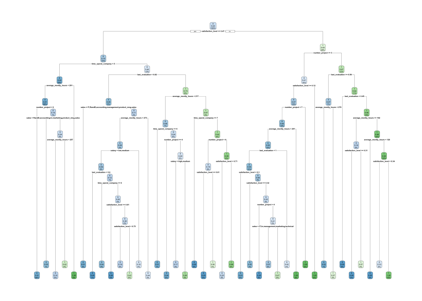
# Examine the complexity plot
printcp(hr_base_model)
##
## Classification tree:
## rpart(formula = left ~ ., data = train, method = "class", control = rpart.control(cp = 0))
##
## Variables actually used in tree construction:
## [1] average_montly_hours last_evaluation number_project
## [4] salary sales satisfaction_level
## [7] time_spend_company
##
## Root node error: 2488/10499 = 0.23697
##
## n= 10499
##
## CP nsplit rel error xerror xstd
## 1 0.23553055 0 1.000000 1.000000 0.0175123
## 2 0.18870579 1 0.764469 0.764469 0.0158619
## 3 0.07616559 3 0.387058 0.387058 0.0118870
## 4 0.05265273 5 0.234727 0.235932 0.0094618
## 5 0.03215434 6 0.182074 0.182476 0.0083768
## 6 0.01406752 7 0.149920 0.150322 0.0076332
## 7 0.01205788 8 0.135852 0.138666 0.0073418
## 8 0.00643087 9 0.123794 0.126608 0.0070257
## 9 0.00522508 10 0.117363 0.121383 0.0068836
## 10 0.00482315 13 0.101688 0.117363 0.0067720
## 11 0.00321543 14 0.096865 0.104502 0.0064002
## 12 0.00281350 15 0.093650 0.096865 0.0061676
## 13 0.00120579 16 0.090836 0.096061 0.0061425
## 14 0.00093783 17 0.089630 0.096463 0.0061551
## 15 0.00048232 20 0.086817 0.097669 0.0061925
## 16 0.00040193 25 0.084405 0.099678 0.0062544
## 17 0.00026795 28 0.083199 0.099678 0.0062544
## 18 0.00011484 31 0.082395 0.103698 0.0063761
## 19 0.00000000 38 0.081592 0.104904 0.0064121plotcp(hr_base_model)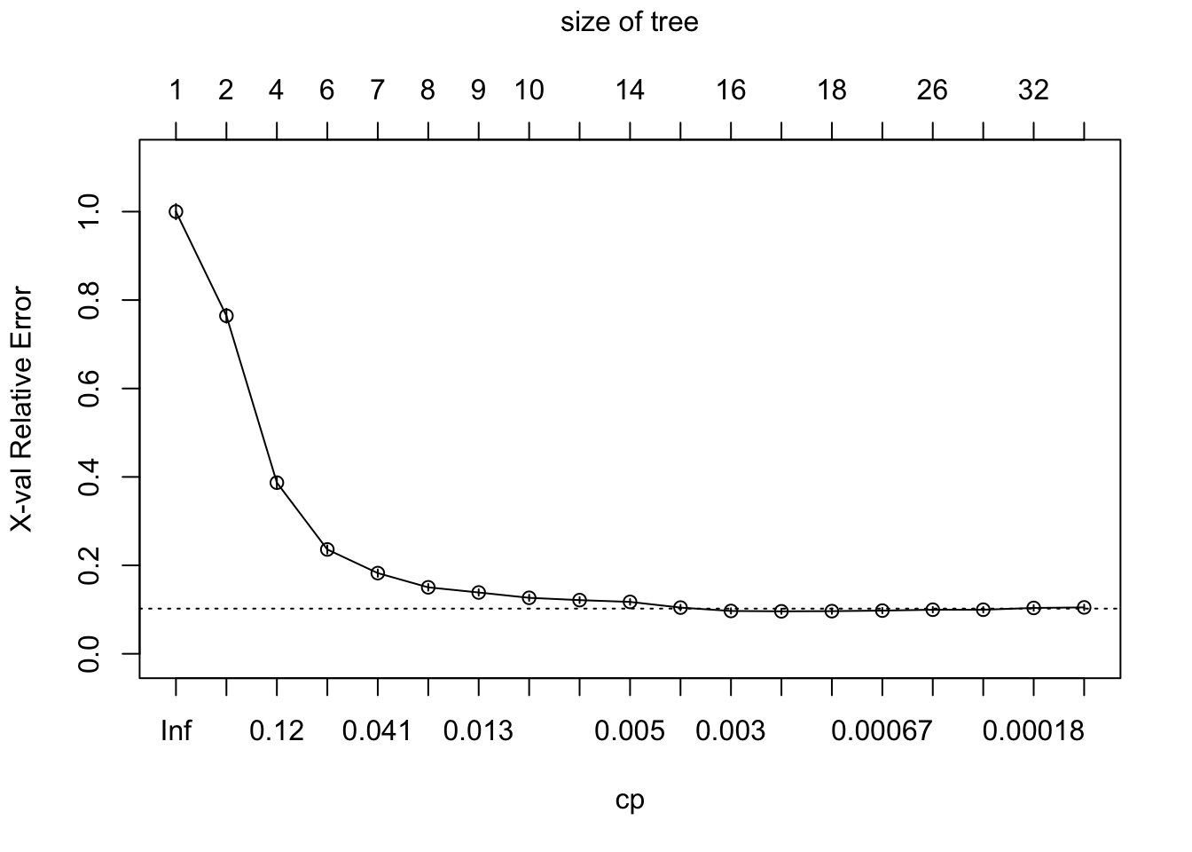
# Compute the accuracy of the pruned tree
test$pred <- predict(hr_base_model, test, type = "class")
base_accuracy <- mean(test$pred == test$left)


# Grow a tree with minsplit of 100 and max depth of 8 (PREPRUNING)
hr_model_preprun <- rpart(left ~ ., data = train, method = "class",
                   control = rpart.control(cp = 0, maxdepth = 8,minsplit = 100))
# Compute the accuracy of the pruned tree
test$pred <- predict(hr_model_preprun, test, type = "class")
accuracy_preprun <- mean(test$pred == test$left)

rpart.plot(hr_model_preprun)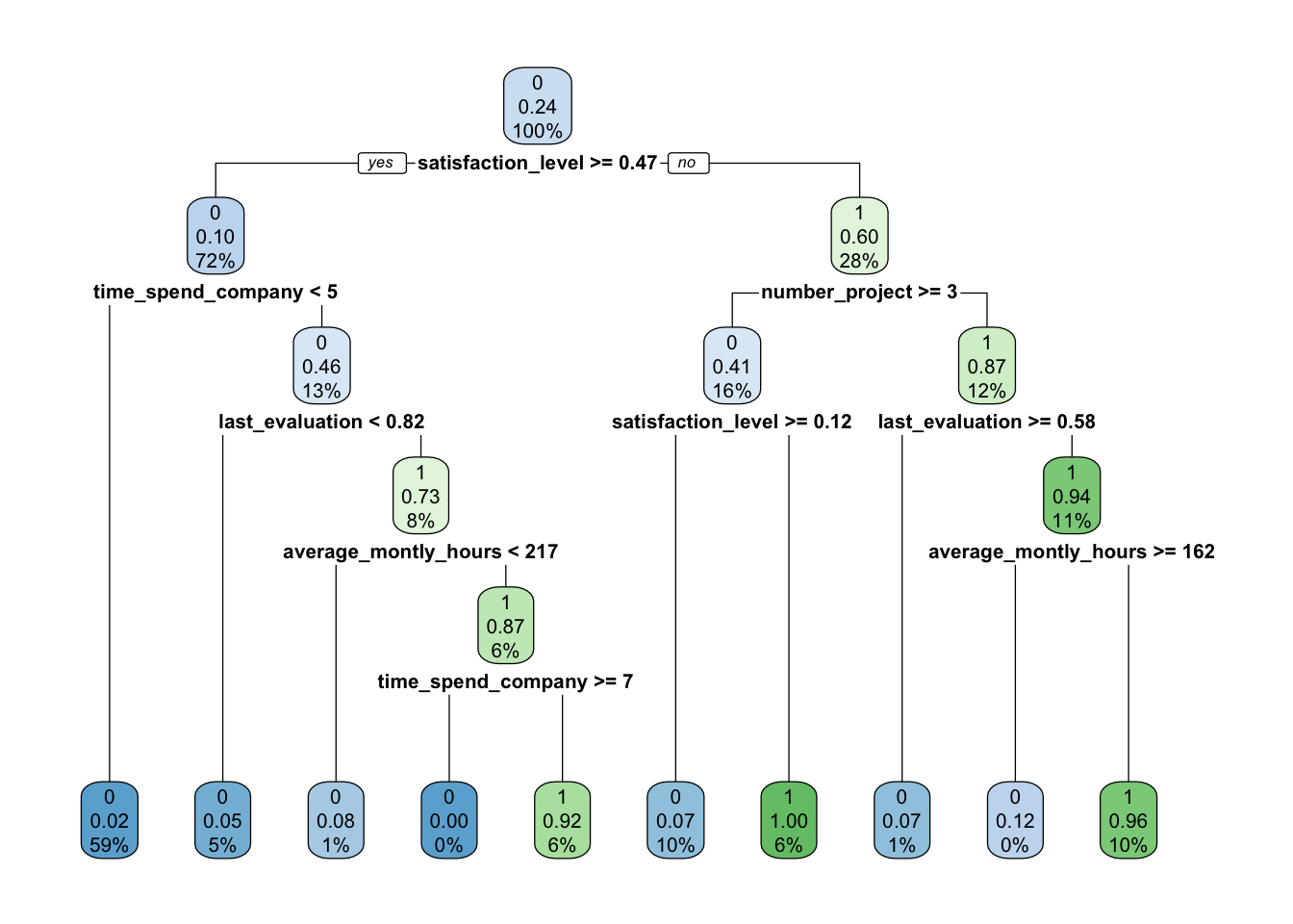
#Postpruning
# Prune the hr_base_model based on the optimal cp value (POSTPRUNING)
hr_model_pruned <- prune(hr_base_model, cp = 0.0046 )
# Compute the accuracy of the pruned tree
test$pred <- predict(hr_model_pruned, test, type = "class")
accuracy_postprun <- mean(test$pred == test$left)

rpart.plot(hr_model_pruned)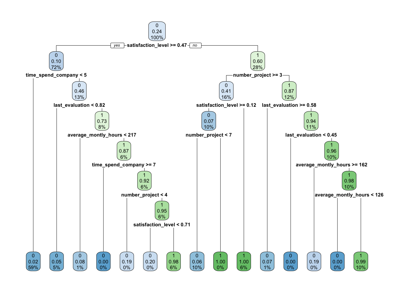
data.frame(base_accuracy, accuracy_preprun, accuracy_postprun)## base_accuracy accuracy_preprun accuracy_postprun
## 1 0.9757778 0.9717778 0.97666674.5 Ejemplo Regresión + Poda
Para este ejemplo necesitaremos instalar algunas librerías
#Librería "AmesHousing"
install.packages("AmesHousing")

#Librería "rsample"
#https://tidymodels.github.io/rsample/
require(devtools) #si no tiene esta librería instalarla
install_github("tidymodels/rsample")

## Librería purrr (functional programming tool - mapping). La forma más sencilla es instalando `tidyverse`
install.packages("tidyverse")
Cargamos las librerías
library(AmesHousing)
library(rsample)     # data splitting
## Loading required package: tidyr##
## Attaching package: 'rsample'## The following object is masked from 'package:tidyr':
##
## filllibrary(dplyr) # data wrangling
library(rpart) # performing regression trees
library(rpart.plot) # plotting regression trees
library(MLmetrics) # goodness of fit##
## Attaching package: 'MLmetrics'## The following object is masked from 'package:base':
##
## RecallPara ilustrar algunos conceptos de regularización vamos usar el conjunto de datos de Ames Housing que se incluye en el paquete del mismo nombre.
# Entrenamiento (70%) y test (30%) a partir de AmesHousing::make_ames() data.
# Usar semilla para reproducibilidad: set.seed

set.seed(123)
ames_split <- initial_split(AmesHousing::make_ames(), prop = .7)
ames_train <- training(ames_split)
ames_test  <- testing(ames_split)
str(ames_train)
## Classes 'tbl_df', 'tbl' and 'data.frame': 2051 obs. of 81 variables:
## $ MS_SubClass : Factor w/ 16 levels "One_Story_1946_and_Newer_All_Styles",..: 1 1 6 6 12 12 6 6 1 6 ...
## $ MS_Zoning : Factor w/ 7 levels "Floating_Village_Residential",..: 3 3 3 3 3 3 3 3 3 3 ...
## $ Lot_Frontage : num 141 93 74 78 41 43 60 75 0 63 ...
## $ Lot_Area : int 31770 11160 13830 9978 4920 5005 7500 10000 7980 8402 ...
## $ Street : Factor w/ 2 levels "Grvl","Pave": 2 2 2 2 2 2 2 2 2 2 ...
## $ Alley : Factor w/ 3 levels "Gravel","No_Alley_Access",..: 2 2 2 2 2 2 2 2 2 2 ...
## $ Lot_Shape : Factor w/ 4 levels "Regular","Slightly_Irregular",..: 2 1 2 2 1 2 1 2 2 2 ...
## $ Land_Contour : Factor w/ 4 levels "Bnk","HLS","Low",..: 4 4 4 4 4 2 4 4 4 4 ...
## $ Utilities : Factor w/ 3 levels "AllPub","NoSeWa",..: 1 1 1 1 1 1 1 1 1 1 ...
## $ Lot_Config : Factor w/ 5 levels "Corner","CulDSac",..: 1 1 5 5 5 5 5 1 5 5 ...
## $ Land_Slope : Factor w/ 3 levels "Gtl","Mod","Sev": 1 1 1 1 1 1 1 1 1 1 ...
## $ Neighborhood : Factor w/ 28 levels "North_Ames","College_Creek",..: 1 1 7 7 17 17 7 7 7 7 ...
## $ Condition_1 : Factor w/ 9 levels "Artery","Feedr",..: 3 3 3 3 3 3 3 3 3 3 ...
## $ Condition_2 : Factor w/ 8 levels "Artery","Feedr",..: 3 3 3 3 3 3 3 3 3 3 ...
## $ Bldg_Type : Factor w/ 5 levels "OneFam","TwoFmCon",..: 1 1 1 1 5 5 1 1 1 1 ...
## $ House_Style : Factor w/ 8 levels "One_Story","One_and_Half_Fin",..: 1 1 6 6 1 1 6 6 1 6 ...
## $ Overall_Qual : Factor w/ 10 levels "Very_Poor","Poor",..: 6 7 5 6 8 8 7 6 6 6 ...
## $ Overall_Cond : Factor w/ 10 levels "Very_Poor","Poor",..: 5 5 5 6 5 5 5 5 7 5 ...
## $ Year_Built : int 1960 1968 1997 1998 2001 1992 1999 1993 1992 1998 ...
## $ Year_Remod_Add : int 1960 1968 1998 1998 2001 1992 1999 1994 2007 1998 ...
## $ Roof_Style : Factor w/ 6 levels "Flat","Gable",..: 4 4 2 2 2 2 2 2 2 2 ...
## $ Roof_Matl : Factor w/ 8 levels "ClyTile","CompShg",..: 2 2 2 2 2 2 2 2 2 2 ...
## $ Exterior_1st : Factor w/ 16 levels "AsbShng","AsphShn",..: 4 4 14 14 6 7 14 7 7 14 ...
## $ Exterior_2nd : Factor w/ 17 levels "AsbShng","AsphShn",..: 11 4 15 15 6 7 15 7 7 15 ...
## $ Mas_Vnr_Type : Factor w/ 5 levels "BrkCmn","BrkFace",..: 5 4 4 2 4 4 4 4 4 4 ...
## $ Mas_Vnr_Area : num 112 0 0 20 0 0 0 0 0 0 ...
## $ Exter_Qual : Factor w/ 4 levels "Excellent","Fair",..: 4 3 4 4 3 3 4 4 4 4 ...
## $ Exter_Cond : Factor w/ 5 levels "Excellent","Fair",..: 5 5 5 5 5 5 5 5 3 5 ...
## $ Foundation : Factor w/ 6 levels "BrkTil","CBlock",..: 2 2 3 3 3 3 3 3 3 3 ...
## $ Bsmt_Qual : Factor w/ 6 levels "Excellent","Fair",..: 6 6 3 6 3 3 6 3 3 3 ...
## $ Bsmt_Cond : Factor w/ 6 levels "Excellent","Fair",..: 3 6 6 6 6 6 6 6 6 6 ...
## $ Bsmt_Exposure : Factor w/ 5 levels "Av","Gd","Mn",..: 2 4 4 4 3 4 4 4 4 4 ...
## $ BsmtFin_Type_1 : Factor w/ 7 levels "ALQ","BLQ","GLQ",..: 2 1 3 3 3 1 7 7 1 7 ...
## $ BsmtFin_SF_1 : num 2 1 3 3 3 1 7 7 1 7 ...
## $ BsmtFin_Type_2 : Factor w/ 7 levels "ALQ","BLQ","GLQ",..: 7 7 7 7 7 7 7 7 7 7 ...
## $ BsmtFin_SF_2 : num 0 0 0 0 0 0 0 0 0 0 ...
## $ Bsmt_Unf_SF : num 441 1045 137 324 722 ...
## $ Total_Bsmt_SF : num 1080 2110 928 926 1338 ...
## $ Heating : Factor w/ 6 levels "Floor","GasA",..: 2 2 2 2 2 2 2 2 2 2 ...
## $ Heating_QC : Factor w/ 5 levels "Excellent","Fair",..: 2 1 3 1 1 1 3 3 1 3 ...
## $ Central_Air : Factor w/ 2 levels "N","Y": 2 2 2 2 2 2 2 2 2 2 ...
## $ Electrical : Factor w/ 6 levels "FuseA","FuseF",..: 5 5 5 5 5 5 5 5 5 5 ...
## $ First_Flr_SF : int 1656 2110 928 926 1338 1280 1028 763 1187 789 ...
## $ Second_Flr_SF : int 0 0 701 678 0 0 776 892 0 676 ...
## $ Low_Qual_Fin_SF : int 0 0 0 0 0 0 0 0 0 0 ...
## $ Gr_Liv_Area : int 1656 2110 1629 1604 1338 1280 1804 1655 1187 1465 ...
## $ Bsmt_Full_Bath : num 1 1 0 0 1 0 0 0 1 0 ...
## $ Bsmt_Half_Bath : num 0 0 0 0 0 0 0 0 0 0 ...
## $ Full_Bath : int 1 2 2 2 2 2 2 2 2 2 ...
## $ Half_Bath : int 0 1 1 1 0 0 1 1 0 1 ...
## $ Bedroom_AbvGr : int 3 3 3 3 2 2 3 3 3 3 ...
## $ Kitchen_AbvGr : int 1 1 1 1 1 1 1 1 1 1 ...
## $ Kitchen_Qual : Factor w/ 5 levels "Excellent","Fair",..: 5 1 5 3 3 3 3 5 5 5 ...
## $ TotRms_AbvGrd : int 7 8 6 7 6 5 7 7 6 7 ...
## $ Functional : Factor w/ 8 levels "Maj1","Maj2",..: 8 8 8 8 8 8 8 8 8 8 ...
## $ Fireplaces : int 2 2 1 1 0 0 1 1 0 1 ...
## $ Fireplace_Qu : Factor w/ 6 levels "Excellent","Fair",..: 3 6 6 3 4 4 6 6 4 3 ...
## $ Garage_Type : Factor w/ 7 levels "Attchd","Basment",..: 1 1 1 1 1 1 1 1 1 1 ...
## $ Garage_Finish : Factor w/ 4 levels "Fin","No_Garage",..: 1 1 1 1 1 3 1 1 1 1 ...
## $ Garage_Cars : num 2 2 2 2 2 2 2 2 2 2 ...
## $ Garage_Area : num 528 522 482 470 582 506 442 440 420 393 ...
## $ Garage_Qual : Factor w/ 6 levels "Excellent","Fair",..: 6 6 6 6 6 6 6 6 6 6 ...
## $ Garage_Cond : Factor w/ 6 levels "Excellent","Fair",..: 6 6 6 6 6 6 6 6 6 6 ...
## $ Paved_Drive : Factor w/ 3 levels "Dirt_Gravel",..: 2 3 3 3 3 3 3 3 3 3 ...
## $ Wood_Deck_SF : int 210 0 212 360 0 0 140 157 483 0 ...
## $ Open_Porch_SF : int 62 0 34 36 0 82 60 84 21 75 ...
## $ Enclosed_Porch : int 0 0 0 0 170 0 0 0 0 0 ...
## $ Three_season_porch: int 0 0 0 0 0 0 0 0 0 0 ...
## $ Screen_Porch : int 0 0 0 0 0 144 0 0 0 0 ...
## $ Pool_Area : int 0 0 0 0 0 0 0 0 0 0 ...
## $ Pool_QC : Factor w/ 5 levels "Excellent","Fair",..: 4 4 4 4 4 4 4 4 4 4 ...
## $ Fence : Factor w/ 5 levels "Good_Privacy",..: 5 5 3 5 5 5 5 5 1 5 ...
## $ Misc_Feature : Factor w/ 6 levels "Elev","Gar2",..: 3 3 3 3 3 3 3 3 5 3 ...
## $ Misc_Val : int 0 0 0 0 0 0 0 0 500 0 ...
## $ Mo_Sold : int 5 4 3 6 4 1 6 4 3 5 ...
## $ Year_Sold : int 2010 2010 2010 2010 2010 2010 2010 2010 2010 2010 ...
## $ Sale_Type : Factor w/ 10 levels "COD","CWD","Con",..: 10 10 10 10 10 10 10 10 10 10 ...
## $ Sale_Condition : Factor w/ 6 levels "Abnorml","AdjLand",..: 5 5 5 5 5 5 5 5 5 5 ...
## $ Sale_Price : int 215000 244000 189900 195500 213500 191500 189000 175900 185000 180400 ...
## $ Longitude : num -93.6 -93.6 -93.6 -93.6 -93.6 ...
## $ Latitude : num 42.1 42.1 42.1 42.1 42.1 ...Para crear el árbol de decisión vamos a usar la misma función rpart como en los ejemplos anteriores,sin embargo se cambia la definición de
method = "anova".La descripción del resultado de la variable
m1puede ser muy extensa, esta muestra la estructura explicativa del árbol generado.
Nota:
- yval = valor medio de las observaciones en el nodo
- deviance = SSE (Sum Square Error) en el nodo
m1 <- rpart(
  formula = Sale_Price ~ .,
  data    = ames_train,
  method  = "anova"
  )
m1
## n= 2051
##
## node), split, n, deviance, yval
## * denotes terminal node
##
## 1) root 2051 1.329920e+13 181620.20
## 2) Overall_Qual=Very_Poor,Poor,Fair,Below_Average,Average,Above_Average,Good 1699 4.001092e+12 156147.10
## 4) Neighborhood=North_Ames,Old_Town,Edwards,Sawyer,Mitchell,Brookside,Iowa_DOT_and_Rail_Road,South_and_West_of_Iowa_State_University,Meadow_Village,Briardale,Northpark_Villa,Blueste 1000 1.298629e+12 131787.90
## 8) Overall_Qual=Very_Poor,Poor,Fair,Below_Average 195 1.733699e+11 98238.33 *
## 9) Overall_Qual=Average,Above_Average,Good 805 8.526051e+11 139914.80
## 18) First_Flr_SF< 1150.5 553 3.023384e+11 129936.80 *
## 19) First_Flr_SF>=1150.5 252 3.743907e+11 161810.90 *
## 5) Neighborhood=College_Creek,Somerset,Northridge_Heights,Gilbert,Northwest_Ames,Sawyer_West,Crawford,Timberland,Northridge,Stone_Brook,Clear_Creek,Bloomington_Heights,Veenker,Green_Hills 699 1.260199e+12 190995.90
## 10) Gr_Liv_Area< 1477.5 300 2.472611e+11 164045.20 *
## 11) Gr_Liv_Area>=1477.5 399 6.311990e+11 211259.60
## 22) Total_Bsmt_SF< 1004.5 232 1.640427e+11 192946.30 *
## 23) Total_Bsmt_SF>=1004.5 167 2.812570e+11 236700.80 *
## 3) Overall_Qual=Very_Good,Excellent,Very_Excellent 352 2.874510e+12 304571.10
## 6) Overall_Qual=Very_Good 254 8.855113e+11 273369.50
## 12) Gr_Liv_Area< 1959.5 155 3.256677e+11 247662.30 *
## 13) Gr_Liv_Area>=1959.5 99 2.970338e+11 313618.30 *
## 7) Overall_Qual=Excellent,Very_Excellent 98 1.100817e+12 385440.30
## 14) Gr_Liv_Area< 1990 42 7.880164e+10 325358.30 *
## 15) Gr_Liv_Area>=1990 56 7.566917e+11 430501.80
## 30) Neighborhood=College_Creek,Edwards,Timberland,Veenker 8 1.153051e+11 281887.50 *
## 31) Neighborhood=Old_Town,Somerset,Northridge_Heights,Northridge,Stone_Brook 48 4.352486e+11 455270.80
## 62) Total_Bsmt_SF< 1433 12 3.143066e+10 360094.20 *
## 63) Total_Bsmt_SF>=1433 36 2.588806e+11 486996.40 *Visualicemos el árbol usando rpart.plot. Este árbol particiona usando 11 varibles, sin embargo hay 80 variables en el conjunto de entrenamiento. ¿Por qué?
rpart.plot(m1)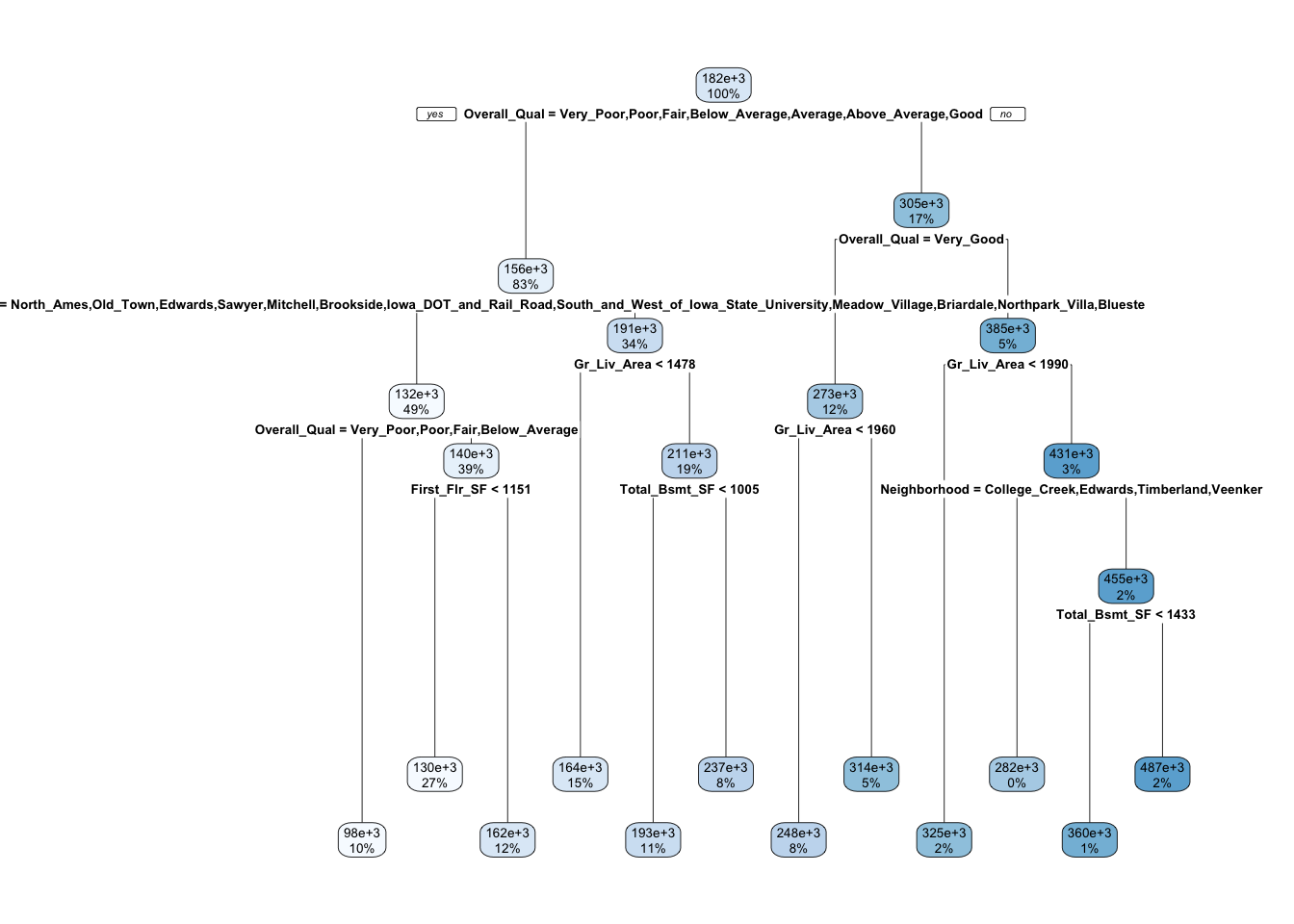
Por defecto rpart aplica un proceso para calcular la penalización de acuerdo al número de árboles.
plotcp(m1)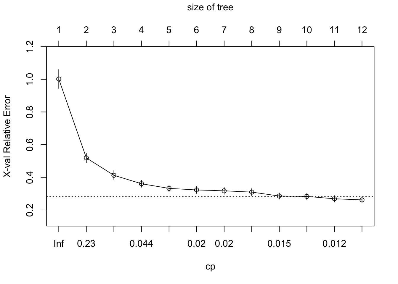
El árbol extendido al máximo, forzando el argumento cp=0
m2 <- rpart(
    formula = Sale_Price ~ .,
    data    = ames_train,
    method  = "anova",
    control = list(cp = 0, xval = 10)
)

plotcp(m2)
abline(v = 12, lty = "dashed")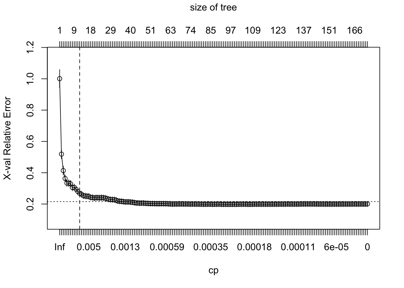
Entonces rpart aplica automáticamente el proceso de optimización para identificar un subárbol óptimo. Para este caso 11 divisiones, 12 nodos terminales y un error de validación cruzada de 0.272. Sin embargo es posible mejorar el modelo a través de un tuning de los parámetros de restricción (e.g., profundidad, número mínimo de observaciones, etc)
m1$cptable## CP nsplit rel error xerror xstd
## 1 0.48300624 0 1.0000000 1.0017486 0.05769371
## 2 0.10844747 1 0.5169938 0.5189120 0.02898242
## 3 0.06678458 2 0.4085463 0.4126655 0.02832854
## 4 0.02870391 3 0.3417617 0.3608270 0.02123062
## 5 0.02050153 4 0.3130578 0.3325157 0.02091087
## 6 0.01995037 5 0.2925563 0.3228913 0.02127370
## 7 0.01976132 6 0.2726059 0.3175645 0.02115401
## 8 0.01550003 7 0.2528446 0.3096765 0.02117779
## 9 0.01397824 8 0.2373446 0.2857729 0.01902451
## 10 0.01322455 9 0.2233663 0.2833382 0.01936841
## 11 0.01089820 10 0.2101418 0.2687777 0.01917474
## 12 0.01000000 11 0.1992436 0.2621273 0.01957837Un ejemplo con algunos valores para probar
m3 <- rpart(
    formula = Sale_Price ~ .,
    data    = ames_train,
    method  = "anova",
    control = list(minsplit = 10, maxdepth = 12, xval = 10)
)

m3$cptable
## CP nsplit rel error xerror xstd
## 1 0.48300624 0 1.0000000 1.0007911 0.05768347
## 2 0.10844747 1 0.5169938 0.5192042 0.02900726
## 3 0.06678458 2 0.4085463 0.4140423 0.02835387
## 4 0.02870391 3 0.3417617 0.3556013 0.02106960
## 5 0.02050153 4 0.3130578 0.3251197 0.02071312
## 6 0.01995037 5 0.2925563 0.3151983 0.02095032
## 7 0.01976132 6 0.2726059 0.3106164 0.02101621
## 8 0.01550003 7 0.2528446 0.2913458 0.01983930
## 9 0.01397824 8 0.2373446 0.2750055 0.01725564
## 10 0.01322455 9 0.2233663 0.2677136 0.01714828
## 11 0.01089820 10 0.2101418 0.2506827 0.01561141
## 12 0.01000000 11 0.1992436 0.2480154 0.01583340Es posbile probar varias combinaciones para encontrar el óptimo a tráves de una búsqueda tipo grid search par encontrar el conjunto óptimo de hyper-parámetros.
Aquí una grilla de valores de minsplit de 5-20 y maxdepth de 8-15. Esto resulta en 128 modelos diferentes.
hyper_grid <- expand.grid(
  minsplit = seq(5, 20, 1),
  maxdepth = seq(8, 15, 1)
)

head(hyper_grid)
## minsplit maxdepth
## 1 5 8
## 2 6 8
## 3 7 8
## 4 8 8
## 5 9 8
## 6 10 8nrow(hyper_grid)## [1] 128Creamos una lista de modelos
models <- list()

for (i in 1:nrow(hyper_grid)) {

  # get minsplit, maxdepth values at row i
  minsplit <- hyper_grid$minsplit[i]
  maxdepth <- hyper_grid$maxdepth[i]

  # train a model and store in the list
  models[[i]] <- rpart(
    formula = Sale_Price ~ .,
    data    = ames_train,
    method  = "anova",
    control = list(minsplit = minsplit, maxdepth = maxdepth)
    )
}
Ahora creamos funciones para extraer el mínimo error asociado con el valor óptimo de costo de complejidad (CP) de cada modelo y adicionalmente el valor óptimo CP y su respectivo error. Agregaremos estos resultados a nuestra grilla de hyper-parámetros y filtraremos los 5 valores con error mínimo.
(xerror of 0.242 versus 0.272).
# function to get optimal cp
get_cp <- function(x) {
  min    <- which.min(x$cptable[, "xerror"])
  cp <- x$cptable[min, "CP"]
}

# function to get minimum error
get_min_error <- function(x) {
  min    <- which.min(x$cptable[, "xerror"])
  xerror <- x$cptable[min, "xerror"]
}

hyper_grid %>%
  mutate(
    cp    = purrr::map_dbl(models, get_cp),
    error = purrr::map_dbl(models, get_min_error)
    ) %>%
  arrange(error) %>%
  top_n(-5, wt = error)
## minsplit maxdepth cp error
## 1 5 13 0.0108982 0.2421256
## 2 6 8 0.0100000 0.2453631
## 3 12 10 0.0100000 0.2454067
## 4 8 13 0.0100000 0.2459588
## 5 19 9 0.0100000 0.2460173Ahora podemos generar nuestro óptimo en base a la información anterior.
optimal_tree <- rpart(
    formula = Sale_Price ~ .,
    data    = ames_train,
    method  = "anova",
    control = list(minsplit = 8, maxdepth = 11, cp = 0.01)
    )

pred <- predict(optimal_tree, newdata = ames_test)
rmse_gof = (MSE(y_pred = pred, y_true = ames_test$Sale_Price))^(1/2)
rmse_gof
## [1] 39145.39rpart.plot(optimal_tree)