6.3 Principal component analysis

Let’s retain only two components or factors:

summary(full_factor(toothpaste, dimensions, nr_fact = 2)) # Ask for two factors by filling in the nr_fact argument.

## Factor analysis
## Data        : toothpaste 
## Variables   : prevents_cavities, shiny_teeth, strengthens_gums, freshens_breath, decay_prevention_unimportant, attractive_teeth 
## Factors     : 2 
## Method      : PCA 
## Rotation    : varimax 
## Observations: 60 
## Correlation : Pearson
## 
## Factor loadings:
##                                RC1   RC2
## prevents_cavities             0.96 -0.03
## shiny_teeth                  -0.05  0.85
## strengthens_gums              0.93 -0.15
## freshens_breath              -0.09  0.85
## decay_prevention_unimportant -0.93 -0.08
## attractive_teeth              0.09  0.88
## 
## Fit measures:
##               RC1  RC2
## Eigenvalues  2.69 2.26
## Variance %   0.45 0.38
## Cumulative % 0.45 0.82
## 
## Attribute communalities:                                   
## prevents_cavities            92.59%
## shiny_teeth                  72.27%
## strengthens_gums             89.36%
## freshens_breath              73.91%
## decay_prevention_unimportant 87.78%
## attractive_teeth             79.01%
## 
## Factor scores (max 10 shown):
##    RC1   RC2
##   1.15 -0.30
##  -1.17 -0.34
##   1.29 -0.86
##   0.29  1.11
##  -1.43 -1.49
##   0.97 -0.31
##   0.39 -0.94
##   1.33 -0.03
##  -1.02 -0.64
##  -1.31  1.56

6.3.1 Factor loadings

Have a look at the table under the header Factor loadings. These loadings are the correlations between the original dimensions (prevents_cavities, shiny_teeth, etc.) and the two factors that are retained (RC1 and RC2). We see that prevents_cavities, strengthens_gums, and decay_prevention_unimportant score highly on the first factor, whereas shiny_teeth, strengthens_gums, and freshens_breath score highly on the second factor. We could therefore say that the first factor describes health-related concerns and that the second factor describes appearance-related concerns.

We also want to know how much each of the six dimensions are explained by the extracted factors. For this, we can look at the communality of the dimensions (header: Attribute communalities). The communality of a variable is the percentage of that variable’s variance that is explained by the factors. Its complement is called uniqueness (= 1-communality). Uniqueness could be pure measurement error, or it could represent something that is measured reliably by that particular variable, but not by any of the other variables. The greater the uniqueness, the more likely that it is more than just measurement error. A uniqueness of more than 0.6 is usually considered high. If the uniqueness is high, then the variable is not well explained by the factors. We see that for all dimensions, communality is high and therefore uniqueness is low, so all dimensions are captured well by the extracted factors.

6.3.2 Loading plot and biplot

We can also plot the loadings. For this, we’ll use two packages:

install.packages("FactoMiner")
install.packages("factoextra")
library(FactoMineR)
library(factoextra)

toothpaste %>% # take dataset
  select(-consumer,-age,-gender) %>% # retain only the dimensions
  as.data.frame() %>% # convert into a data.frame object, otherwise PCA won't accept it
  PCA(ncp = 2, graph = FALSE) %>% # do a principal components analysis and retain 2 factors
  fviz_pca_var(repel = TRUE) # take this analysis and turn it into a visualization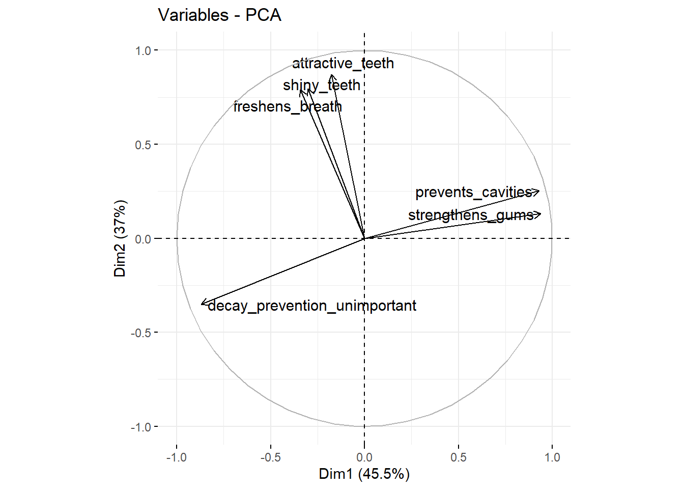

We see that attractive_teeth, shiny_teeth, freshens_breath have high scores on the second factor (the X-axis Dim2). prevents_cavities and strengthens_gums have high scores on the second factor (the Y-axis Dim2) and decay_prevention_unimportant has a low score on this factor (this variable measures how unimportant prevention of decay is). We can also add the observations (the different consumers) to this plot:

toothpaste %>% # take dataset
  select(-consumer,-age,-gender) %>% # retain only the dimensions
  as.data.frame() %>% # convert into a data.frame object, otherwise PCA won't accept it
  PCA(ncp = 2, graph = FALSE) %>% # do a principal components analysis and retain 2 factors
  fviz_pca_biplot(repel = TRUE) # take this analysis and turn it into a visualization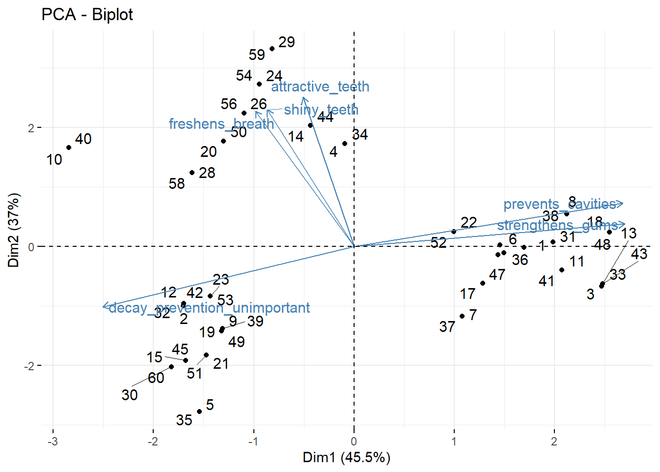

This is also called a biplot.