4.4 Moderation analysis: Interaction between continuous and categorical independent variables
Say we want to test whether the results of the experiment depend on people’s level of dominance. In other words, are the effects of power and audience different for dominant vs. non-dominant participants? In still other words, is there a three-way interaction between power, audience, and dominance?
Let’s create a graph first:
# Our dependent variable is conspicuous consumption, our independent variable (on the X-axis) is dominance.
# So we're plotting the relationship between dominance and conspicuous consumption.
# The color argument tells R that we want a relationship for each level of power.

ggplot(data = powercc, mapping = aes(x = dominance, y = cc, color = power)) +
  facet_wrap(~ audience) + # Tell R that we also want to split up by audience.
  geom_jitter() + # Use geom_jitter instead of geom_point, otherwise the points are drawn over each other
  geom_smooth(method='lm', se=FALSE) # Draw a linear regression line through the points.
## `geom_smooth()` using formula 'y ~ x'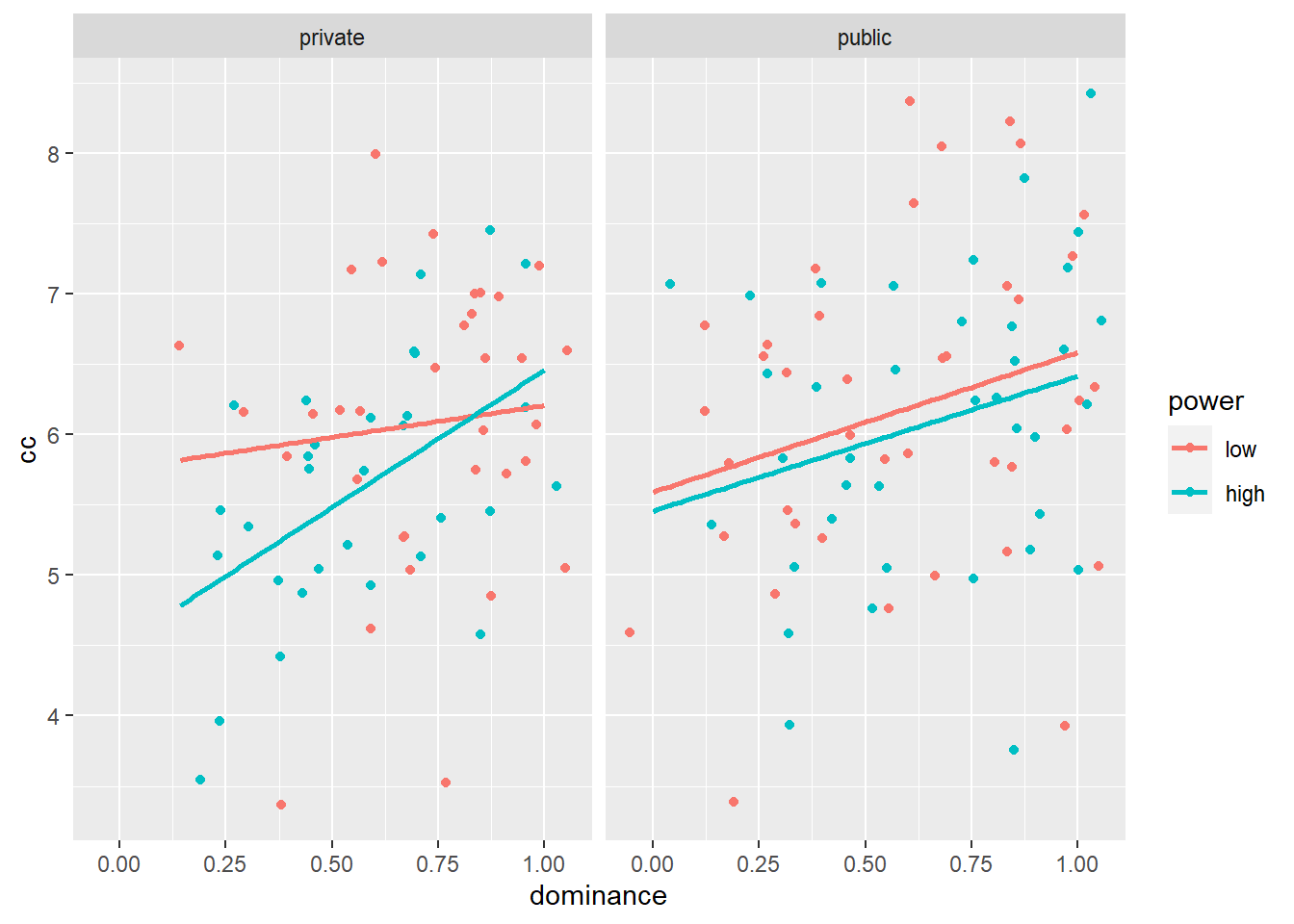
This graph is informative. It shows us that in the private condition, the effect of high vs. low power on conspicuous consumption is more negative for less dominant participants than for more dominant participants. In the public condition, the effect of high vs. low power on conspicuous consumption does not differ between less vs. more dominant participants. We also see that in both the private and the public condition, more vs. less dominant participants are more willing to spend on conspicuous consumption.
Let’s check whether the three-way interaction is significant:
linearmodel <- lm(cc ~ power * audience * dominance, data = powercc)
type3anova(linearmodel)
## # A tibble: 9 x 6
## term ss df1 df2 f pvalue
## <chr> <dbl> <dbl> <int> <dbl> <dbl>
## 1 (Intercept) 525. 1 135 519. 0
## 2 power 2.21 1 135 2.18 0.142
## 3 audience 0.715 1 135 0.706 0.402
## 4 dominance 10.5 1 135 10.3 0.002
## 5 power:audience 1.44 1 135 1.42 0.235
## 6 power:dominance 1.18 1 135 1.17 0.282
## 7 audience:dominance 0.113 1 135 0.111 0.739
## 8 power:audience:dominance 1.30 1 135 1.29 0.258
## 9 Residuals 137. 135 135 NA NAOnly the effect of dominance is significant. If the three-way interaction were significant, we could follow-up with more tests. For example, we could test whether the two-way interaction between dominance and power is significant in the private condition, as the graph suggests. To do this, let’s first take a look at the regression coefficients of our linear model:
summary(linearmodel)##
## Call:
## lm(formula = cc ~ power * audience * dominance, data = powercc)
##
## Residuals:
## Min 1Q Median 3Q Max
## -2.58617 -0.63357 0.09751 0.68310 2.24067
##
## Coefficients:
## Estimate Std. Error t value Pr(>|t|)
## (Intercept) 5.7553 0.6019 9.561 <2e-16 ***
## powerhigh -1.2490 0.7703 -1.621 0.107
## audiencepublic -0.1651 0.6918 -0.239 0.812
## dominance 0.4526 0.7980 0.567 0.572
## powerhigh:audiencepublic 1.1162 0.9355 1.193 0.235
## powerhigh:dominance 1.5021 1.1111 1.352 0.179
## audiencepublic:dominance 0.5434 0.9514 0.571 0.569
## powerhigh:audiencepublic:dominance -1.5394 1.3561 -1.135 0.258
## ---
## Signif. codes: 0 '***' 0.001 '**' 0.01 '*' 0.05 '.' 0.1 ' ' 1
##
## Residual standard error: 1.006 on 135 degrees of freedom
## Multiple R-squared: 0.1225, Adjusted R-squared: 0.07703
## F-statistic: 2.693 on 7 and 135 DF, p-value: 0.01211We have eight terms in our model:
- \(\beta_0\) or the intercept
- \(\beta_1\) or the coefficient for “powerhigh”
- \(\beta_2\) or the coefficient for “audiencepublic”
- \(\beta_3\) or the coefficient for “dominance”
- \(\beta_4\) or the coefficient for “powerhigh:audiencepublic”
- \(\beta_5\) or the coefficient for “powerhigh:dominance”
- \(\beta_6\) or the coefficient for “audiencepublic:dominance”
- \(\beta_7\) or the coefficient for “powerhigh:audiencepublic:dominance”
Resulting in this table of coefficients:
#                     private                         public
# low power          [b0] + (b3)                     [b0+b2] + (b3+b6)
# high power         [b0+b1] + (b3+b5)               [b0+b1+b2+b4] + (b3+b5+b6+b7)
How did we get this table? With the linear model specified above, each estimated value of conspicuous consumption (the dependent variable) is a function the participant’s experimental condition and the participant’s level of dominance. Say we have a participant in the low power, public condition with a level of dominance of 0.5. The estimated value of conspicuous consumption for this participant is:
- \(\beta_0\): intercept \(\times\) 1
- \(\beta_1\): “powerhigh” \(\times\) 0 (because the participant is not in the high power condition)
- \(\beta_2\): “audiencepublic” \(\times\) 1 (in the public condition)
- \(\beta_3\): “dominance” \(\times\) 0.5 (dominance = 0.5)
- \(\beta_4\): “powerhigh:audiencepublic” \(\times\) 0 (not in both the high power & the public condition)
- \(\beta_5\): “powerhigh:dominance” \(\times\) 0 (not in the high power condition)
- \(\beta_6\): “audiencepublic:dominance” \(\times\) 1 \(\times\) 0.5 (in the public condition and dominance = 0.5)
- \(\beta_7\): “powerhigh:audiencepublic:dominance” \(\times\) 0 (not in both the high power & the public condition)
or \(\beta_0\) \(\times\) 1 + \(\beta_1\) \(\times\) 0 + \(\beta_2\) \(\times\) 1 + \(\beta_3\) \(\times\) 0.5 + \(\beta_4\) \(\times\) 0 + \(\beta_5\) \(\times\) 0 + \(\beta_6\) \(\times\) 0.5 + \(\beta_7\) \(\times\) 0
= [\(\beta_0\) + \(\beta_2\)] + (\(\beta_3\) + \(\beta_6\)) \(\times\) 0.5
= [5.76 + -0.17] + (0.45 + 0.54) * 0.5 = 6.09
Check the graph to see that this indeed corresponds to the estimated conspicuous consumption of a participant with dominance = 0.5 in the low power, public cell.
The general formula for the low power, public cell is the following:
[\(\beta_0\) + \(\beta_2\)] + (\(\beta_3\) + \(\beta_6\)) \(\times\) dominance
and we can obtain the formulas for the different cells in a similar manner. We see that in each cell, the coefficient between square brackets is the estimated value on the conspicuous consumption measure for a participant who scores 0 on dominance. The coefficient between round brackets is the estimated increase in the conspicuous consumption measure for every one unit increase in dominance. In other words, the coefficients between square brackets represent the intercept and the coefficients between round brackets represent the slope of the line that represents the regression of conspicuous consumption (Y) on dominance (X) within each experimental cell (i.e., each power & audience combination).
A test of the interaction between power and dominance within the private condition would come down to testing whether the blue and the red line in the left panel of the figure above should be considered parallel or not. If they are parallel, then the effect of dominance on conspicuous consumption is the same in the low and the high power condition. If they’re not parallel, then the effect of dominance is different in the low versus the high power condition. In other words, we should test whether the regression coefficients are equal within low power, private and within high power, private. In still other words, we test whether (\(\beta_3\) + \(\beta_5\)) - \(\beta_3\) = \(\beta_5\) is equal to zero:
# now we have eight numbers corresponding to the eight regression coefficients
# we want to test whether b5 is significant, so we put a 1 in 6th place (1st place is for b0)
contrast_specification <- c(0, 0, 0, 0, 0, 1, 0, 0)

contrast(linearmodel, contrast_specification)
##
## Simultaneous Tests for General Linear Hypotheses
##
## Fit: aov(formula = linearmodel)
##
## Linear Hypotheses:
## Estimate Std. Error t value Pr(>|t|)
## 1 == 0 1.502 1.111 1.352 0.179
## (Adjusted p values reported -- single-step method)The interaction is not significant, however. You could report this as follows: “Within the private condition, there was no interaction between power and dominance (t(135) = 1.352, p = 0.18).”
4.4.1 Spotlight analysis
Coming soon.