4 Statistical Inference - Case Study Satisfaction with Government
4.1 Introduction
In Western democracies, citizens’ satisfaction with the government is critically related to the electoral success of governing parties in an upcoming election. At the same time, satisfied citizens are more willing to support non-preferred policies and are less likely to support anti-system or populist parties.
If we are interested in the degree of satisfaction with the government in Germany, for example, we first need to define the population we aim to make statements about (e.g., people over 18 years old who live in Germany). Conducting interviews with each person that belongs to the population would be pointless. Instead, we can rely on the “shortcut” of random sampling, in which we randomly select observational units from this population (i.e., randomly selected Germans) and survey them. The idea is that the results (e.g., mean approval of the government using a survey item) from the random sample are representative of the underlying population - that is, a close match between the parameter estimated from the sample (e.g., mean approval) and the (unobserved) parameter of the population.

In statistical inference, we are primarily interested in how accurately an estimate from a sample reflects the true population parameter. Thus, the goal is to find a suitable measure of precision (or uncertainty, as the other “side of the coin”). We do this by matching the estimate from the sample with a test distribution that reflects likely or unlikely values in terms of probabilities. How this is done will be discussed in this case study.
Before that, we take a short excursion into the realm of probability theory.
4.2 Probability
Probabilities correspond to the ratio of the number of observations that meet a certain criterion (i.e., an “event”) to the total number of observations. A classic example is the coin toss and the ratio between heads and the total number of tosses. Probabilities are always positive (\(P(A)\ge0\)). The probability of all possible events (e.g., heads and tails in the case of a coin toss) is 1 (\(P(\Omega)=1\)). If events A and B cannot occur simultaneously, then the probability of A or B occurring is the summed probability for both events (\(P(A or B)=P(A)+P(B)\)).
The probabilities of events that occur in a chance experiment (e.g., a coin toss) can be represented as so-called random variables. Random variables have a probability distribution, for binary variables (0/1) this is the Bernoulli distribution, for continuous variables this is the normal distribution. (There are other distributions like the F-distribution or chi-square distribution, which we will use later for further purposes).
Here we see a probability distribution for 10 balls (7 blue, 3 red) randomly drawn with replacement, in total 10,000 draws were made. Accordingly, the probability distribution is approximately 0.7 for blue and 0.3 for red:
possible_values <- c(1,0)
Bernoulli <- sample(possible_values,
               size=10000,
               replace=TRUE,
               prob=c(0.3, 0.7))
prop.table(table(Bernoulli))
## Bernoulli
## 0 1
## 0.7034 0.2966
h <- hist(Bernoulli,plot=FALSE)
h$density = h$counts/sum(h$counts)*100
plot(h,freq=FALSE, axes=FALSE)
axis(1, at = c(0, 1), labels = c("Blue", "Red"))
axis(2, at = c(0, 10, 20, 30, 40, 50, 60, 70))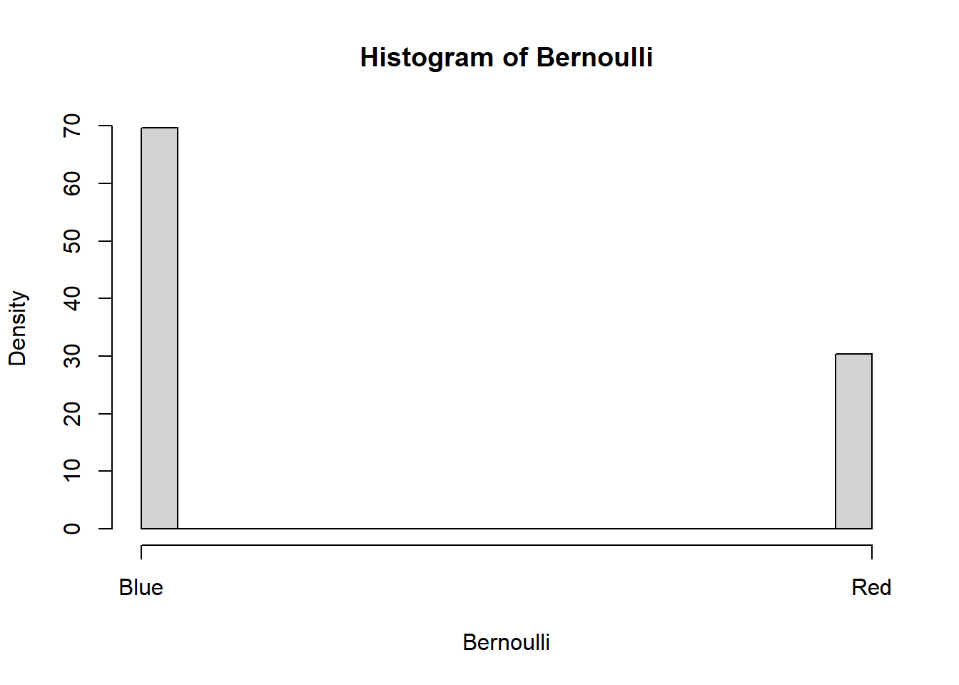
The Bernoulli distribution is characterized by the probability of occurrence of an event \(p\). The probability for the counter-event automatically follows from this: \(1-p\). We will need this distribution for the calculation of test statistics of proportions.
The normal distribution for random variables is a bell-shaped probability density function. It gives the probabilities for a continuous random variable with infinite intermediate values. Think of time as a continuous concept. Theoretically, we can measure time in infinitely small units (milliseconds, nanoseconds, etc.). However, in applied research, we would assign discrete values to the variable time. Hence, continuous variables are rather a theoretical concept. Regarding the distribution of a continuous random variable: The normal distribution is characterized by a mean \(\mu\) and a standard deviation \(\sigma\). The notation for the normal distribution of a random variable is \(X \sim N(\mu,\sigma)\). Each combination of \(\mu\) and \(\sigma\) gives a differently shaped normal distribution. The mean indicates where the center of the distribution is on the x-axis and \(\sigma\) indicates how flat or steep the distribution is (the higher, the more spread out and thus the flatter the curve becomes).
The so-called standard normal distribution has a mean of 0 and a standard deviation of 1 (\(X \sim N(0,1)\)). As with all other normal distributions, (1) the ends of the curve spread out to the left and right, approaching the x-axis without ever touching it. Thus, the values can range from - to + infinity. (2) The area under the curve is equal to 1 in total. (3) The so-called “Empirical Rule” states that for a standard normal distribution, 68% of the observations lie between -1 and +1 standard deviations. 95% of the observations lie between approx. -2 and +2 standard deviations (to be exact -1.96 and +1.96), and 99.7% of the observations lie between approximately -3 and +3 standard deviations.
# Draw a standard normal distribution:
z = seq(-4, 4, length.out=1001)
x = rnorm(z)
plot( x=z, y=dnorm(z), bty='n', type='l', main="Standard normal distribution", ylab="Probability density", xlab="z", xlim=c(-3,3))
axis(1, at = seq(-4, 4, by = 1))

# annotate the density function with the 5% probability mass tails
polygon(x=c(z[z<=qnorm(0.025)], qnorm(0.025), min(z)), y=c(dnorm(z[z<=qnorm(0.025)]), 0, 0), col=grey(0.8))
polygon(x=c(z[z>=qnorm(0.975)], max(z), qnorm(0.975)), y=c(dnorm(z[z>=qnorm(0.975)]), 0, 0), col=grey(0.8))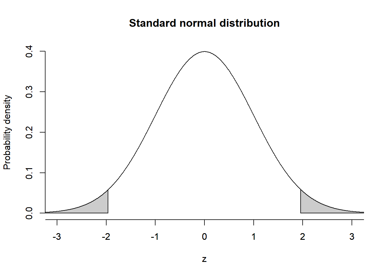
With probability distributions such as the standard normal distribution, we do not calculate the probability of a specific value but rather a range of values. For example, the probability that a value is greater than 1.96 standard deviations, i.e., \(P(Z\ge1.96)\), is 2.5%. And the probability that a value is less than -1.96 standard deviations, i.e., \(P(Z\le-1.96)\), is 2.5% (see the grey areas in the plot above, both areas sum up to 5%).
We will use the standard normal distribution (also referred to as Z-distribution) for various statistical tests. The rule that 95% of observable values are located between -1.96 and 1.96, and 5% at the outer margins will also become important in Null Hypothesis Testing.
4.3 Basics of statistical inference
Inference means that we use facts we know to learn about facts we don’t know (yet). Statistical inference means that we take information from a (random) sample and infer from it (not yet known) properties of the population (from which the sample was drawn). Basically, only random samples are suitable for this purpose, since they represent the underlying population in all properties in the best possible way (plus minus some random variation).
While random samples are the best way to conduct statistical inference, the process is not flawless. There is still a chance that the units in our sample do not perfectly match all properties of the population due to random deviations. It may be that a sample was drawn in which disproportionately many women accidentally “slipped in”. These random deviations are called sampling variability. The following sections should illustrate that sampling variability decreases with the number of observations in a sample (“more data is better”) and that if we did the process of random sampling over and over again (with a sufficiently large number of observations), we would obtain a distribution of sampled estimates that are shaped like a normal distribution. This will be tremendously useful when we conduct statistical tests, in which we use the normal distribution as if it was the sampling distribution of a quantity of interest we can match and test our estimate with.
4.3.1 Law of Large Numbers
In general, a small number of cases leads to higher sampling variability. You may be familiar with this from the coin toss experiment. A coin is often tossed in succession. After 10 tosses, it is quite possible that heads were tossed 7 times and tails only 3 times. Nevertheless, the underlying probability is always 0.5/0.5 (or 50%/50%) and in the population of all coin tosses, heads and tails should occur equally often. If we now toss the coin even more often, after 30, 300, 3000, etc. the observed coin tosses will increasingly match the 0.5/0.5 probability distribution.
The law of large numbers states that as the sample size increases, the mean of the sample will increasingly approxiamte that of the population. (Eventually, the sample would be identical to the entire population.) This means that more data is better, and the larger our sample, the more confident we can be that it matches or at least approximates the population parameter.
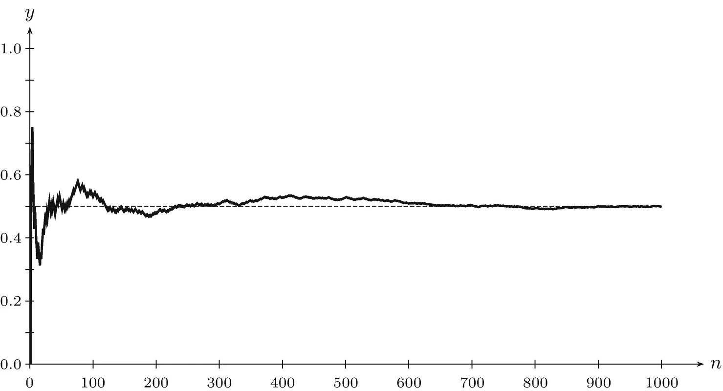
Source: https://link.springer.com/chapter/10.1007/978-3-030-45553-8_5
4.3.2 Central Limit Theorem
If we draw many (or even infinite) samples from a population and are interested in, for example, the mean of satisfaction with government, then plotting the means of each sample as a histogram will lead to a distribution that (with added samples increasingly) follows a normal distribution. The mean of the sample means thereby corresponds to the population parameter we are essentially interested in (i.e., satisfaction with the government of all over-18-year-olds living in Germany).
The implications of the central limit theorem are illustrated in the following figure. The mean of the means from 100,000 simulated samples is 4.2 and corresponds to the “true” population mean of government satisfaction. Note that in reality, we do not have this information and we are not able to draw these many samples as that would be too costly.
set.seed(123)
data <- rnorm(100000, 4.2, 1)
hist(data, freq = FALSE, col = "gray", xlab = "Data Values", main = "Means of government satisfaction")
curve(dnorm(x, mean = mean(data), sd = sd(data)), col = "black", lwd = 2, add = TRUE)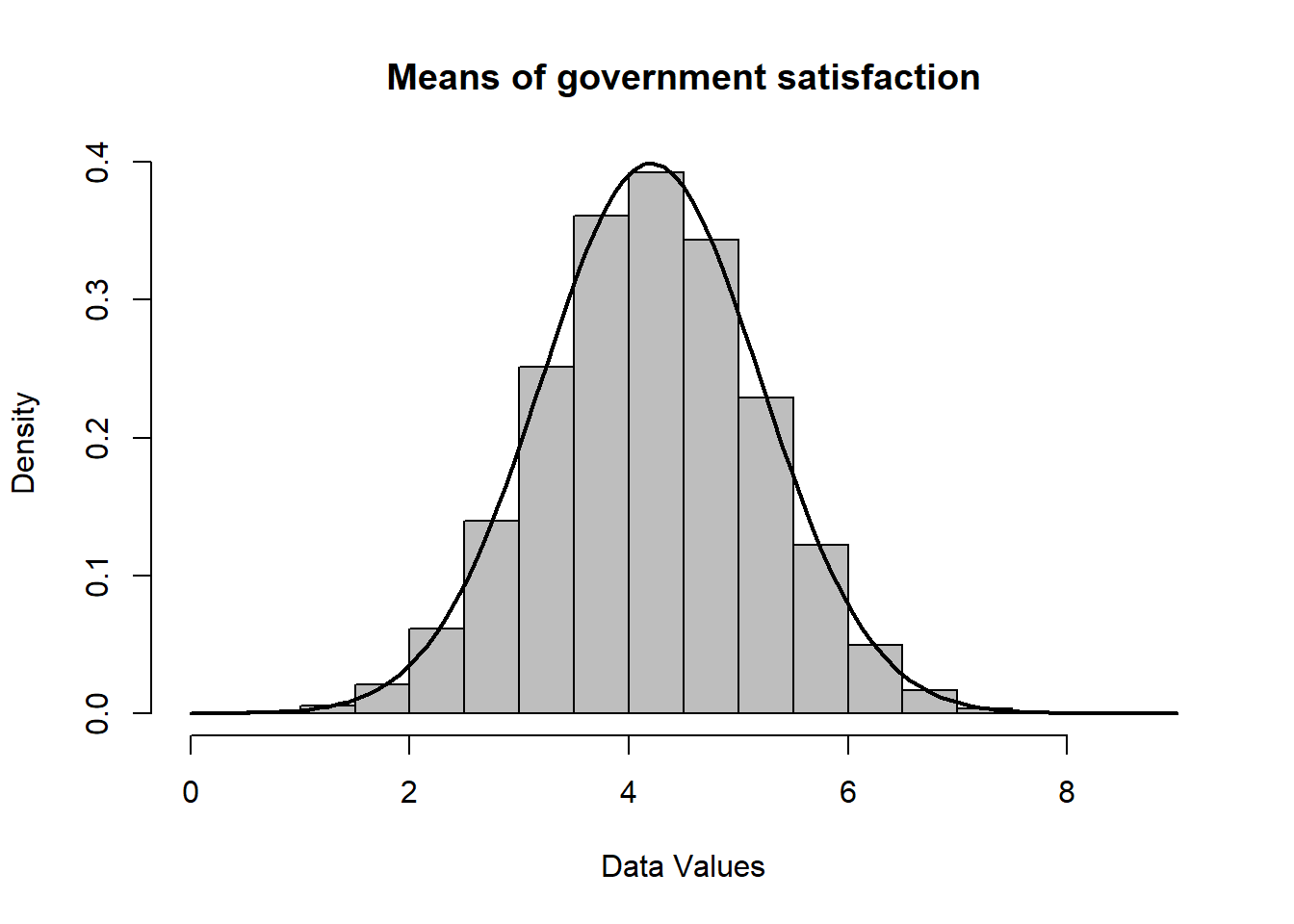
Another property of the central limit theorem is that the larger the number of cases (\(n\)) of each of the individual samples, the better the distribution of sample estimates corresponds to a normal distribution. This works very well with \(n>30\). Moreover, it is not important how the distribution of the characteristic to be examined is in the population (e.g., right- or left-skewed). In any case, with increasing samples (and \(n>30\)), the distribution of sample estimates will (with added samples increasingly) correspond to a normal distribution.
4.3.3 Why statistical laws are important
4.3.3.1 Only one sample
We calculate everything on the basis of one sample, everything else would be too costly.
-
We can never be completely sure that the ONE specific sample and the statistics estimated using it correspond to those of the population, but:
The larger the sample, the steeper the distribution of sample estimates and the more certain we are to get an estimated parameter near the population parameter, even with only one sample (Law of Large Numbers).
For a sample of 30 or more observations, we know that the distribution of sample estimates is normal no matter how the distribution of the population looks like; this gives us the rationale that most samples mingle around the population mean and that there is quite a high probability that the estimate from our one sample is near the center of the distribution (i.e., close to the population parameter); getting an estimate that is far away from the center of the distribution is rather unlikely (Central Limit Theorem).
4.3.3.2 A Primer on Null Hypothesis Testing
The Central Limit Theorem also gives us a rationale for quantifying uncertainty, because if repeated sample estimates can be represented as a normal distribution, then we can use the normal distribution as a frame of reference for how credible the results from our one sample are.
To do so, we make specific assumptions about the distribution we test our sample estimate against (e.g., a distribution that assumes no difference in means between two groups).
This procedure is called Null Hypothesis Testing (or, NHT):
We develop a research hypothesis or a so-called alternative hypothesis (e.g., women are more satisfied with the government than men).
We use a random sample and estimate the difference in means of government satisfaction between men and women.
We test our result against a (theoretical) distribution under which we assume the null hypothesis (-> there is NO difference in government satisfaction between men and women) to be true (i.e., the test distribution).
If the estimate from our sample is located near the center of the distribution that assumes the null hypothesis, this would be not much evidence for the alternative hypothesis; however: If the estimate is at the margins of that distribution, we would conclude that there is evidence that favor the alternative hypothesis, which states that in the population, women are more satisfied with the government than men.
- The prerequisite for this testing procedure is that we standardize our sample estimate to make it comparable to the test distribution (For example, this can be achieved by: \(z = \frac{estimate}{{standard error}}\)).
4.3.3.3 Standard error
To determine the variation around a population parameter, we could use the standard deviation of the sampling distribution.
However, since in the applied case we do not have many samples, but only one, we need to estimate this variation from the one sample.
This estimated variation of an estimate is called the standard error, and the formula for calculating it differs depending on the estimator (usually we normalize a measure of variance or standard deviation using a measure that involves the number of observations; for example, the standard error of mean the formula is given as: \(\bar x = \frac{s}{\sqrt{n}}\)).
4.4 Confidence intervals
4.4.1 Basic idea
In theory, the confidence intervals (CIs) for a point estimate (e.g., a mean or a correlation coefficient) shows a range of values that contain the true population parameter with a certain probability. It is thus a measure of uncertainty (or, conversely, precision) of an estimate. There are conventionally three types of confidence intervals: 90%, 95%, and 99% confidence intervals. These three types reflect the level of probability that the true population value lies within the interval for a very large number of samples. For example, if one is interested in the population mean and conducts repeated (“infinite”) sampling, 95% of the confidence intervals of the respective samples would contain the true population mean, and 5% would not contain it.
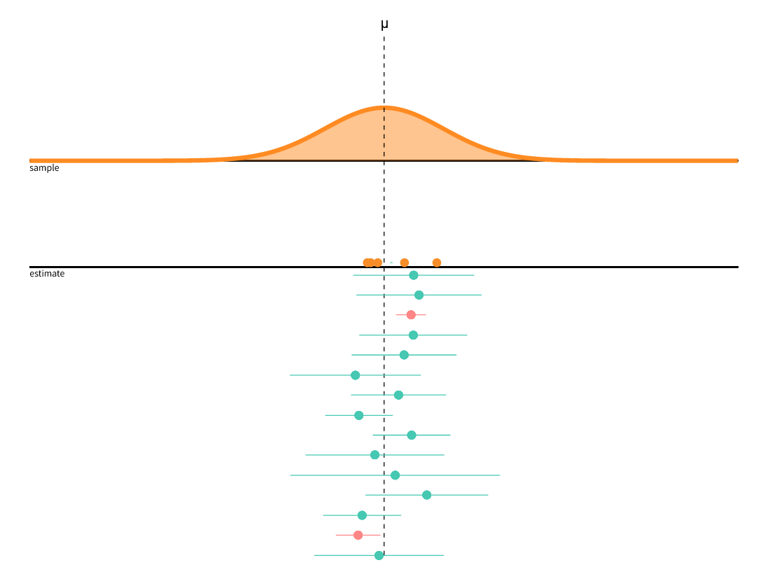
This can be illustrated with the following figures.
Source: https://seeing-theory.brown.edu/frequentist-inference/index.html
In the figure, samples were repeatedly drawn from a population with five observations each (orange dots). Each time, the mean is calculated (or estimated because we are using a sample). These point estimates of the mean from each sample are represented by the green or red dots, the confidence interval is the corresponding line to the left and right of it. For the green estimates, the population mean (dashed line) is within the confidence interval, for the red it is not.
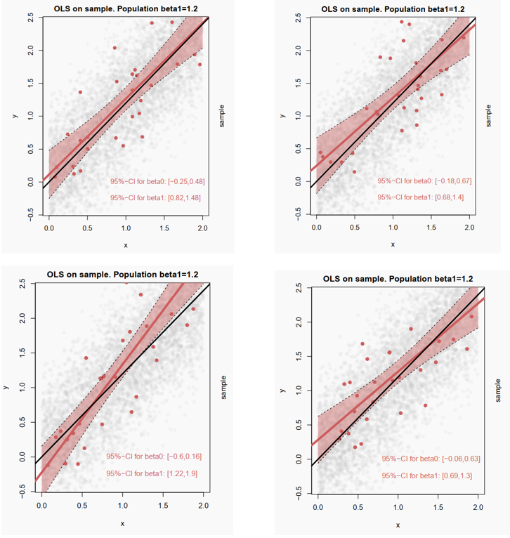
Source: https://github.com/simonheb/metrics1-public
Here, instead of the mean value, results of a bivariate regression (similar to a correlation) are shown. The bivariate relationship between x and y in the population is represented by the black slope line (regression coefficient \(\beta_1=1.2\)). The gray dots are the units in the population. From this population, four random samples are drawn and the observations in the sample are represented by the red dots. The point estimate of the correlation is represented by the red slope line. The confidence interval is the light red area around the estimate. In samples 1, 2, and 4, the confidence interval includes the population parameter; only in sample 3 (bottom left) is this no longer the case for parts of the confidence interval. Analogously to the thought experiment regarding means above, 95% of estimates from repeated samples would include the population mean, and 5% would not.
4.4.2 How to calculate and interpret the confidence interval
The idea of confidence intervals refers to the sampling distribution, i.e. many (up to infinitely many) repeated random samples from the population. For a 95% confidence interval, the interpretation would be: for repeated samples, 95% of the samples will contain the population parameter, 5% will not.
In practice, we only have one sample and can therefore only calculate confidence intervals once. Whether the population parameter actually falls within the value range of the confidence interval of our one sample or not cannot be answered conclusively. What can be said is that the likelihood of this is high. For example, with the 95% confidence interval, 95 out of 100 samples would have to contain the population parameter and it is likely that our one sample is one of the 95 and not one of the 5. (At the same time, some interpretations made in textbooks such as “with 95% probability the population parameter is in the interval” are strictly speaking not true).
We can therefore interpret the confidence intervals primarily as the likely or plausible range of values of the unknown population parameter we are interested in (given the characteristics of our sample). The confidence interval thus gives us, at the same time as the point estimate, a range of variability to be expected if we were to repeat studies similar to ours more often. This is indeed important information, and for many researchers, it is also more intuitive than significance values from null hypothesis tests.
In addition, there is a relationship between confidence intervals and statistical significance, a concept related to null hypothesis tests. We will look at this relationship at the end of this case study. In short, confidence intervals show a possible range of values of the population parameter and at the same time provide information about statistical significance.
To compute a confidence interval, we generally use the following formula:
\(point estimate \pm z_\alpha \times standard error\).
\(z_\alpha\) refers to the critical Z-value (i.e., a given value of the z-distribution that corresponds a set probability of error, this will be explained in greater detail below).
4.4.2.1 Mean
For the lower and upper 95% confidence intervals of a mean, we use: \(95\% CIs=[\bar x - 1.96 \times {\frac{s}{\sqrt n}}, \bar x + 1.96 \times {\frac{s}{\sqrt n}}]\).
Let us look into this with real data from the European Social Survey (German sample). First, we read the data and get an overview of the distribution of the variable satisfaction with government stfgov. stfgov was surveyed using an 11-point scale ranging from 0 “extremely dissatisfied” to 10 “extremely satisfied.”
data_ess <- read_dta("data/ESS9_DE.dta", encoding = "latin1")

hist(data_ess$stfgov, breaks = "FD")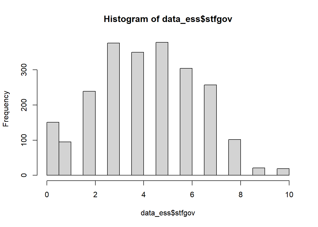
summary(data_ess$stfgov)## Min. 1st Qu. Median Mean 3rd Qu. Max. NA's
## 0.00 3.00 4.00 4.28 6.00 10.00 66Next, we calculate the 95% confidence interval in several steps:
# We store the mean, the standard deviation and the number of observations as objects, because this way we can refer to them later on
n <- 2292
xbar <- mean(data_ess$stfgov, na.rm = TRUE)
s <- sd(data_ess$stfgov, na.rm = TRUE)

# Set confidence level with 1-alpha (alpha = our willingness to be wrong in repeated samples)
conf.level <- 0.95

# Calculating the critical z-value for a two-sided test
z <- qnorm((1 + conf.level) / 2)

# Calculate the confidence interval
lower.ci <- xbar - z * s / sqrt(n)
upper.ci <- xbar + z * s / sqrt(n)

# Print confidence intervals
cat("The", conf.level*100,"% confidence interval for the population mean is (",round(lower.ci, 2), ",", round(upper.ci, 2),").\n")
## The 95 % confidence interval for the population mean is ( 4.19 , 4.37 ).Computing confidence intervals is even easier with the “t.test” command. While we are interested in the z-distribution, t- and z-distribution correspond to each other when the number of observations is high enough (usually already >30).
Let’s try it out:
t.test(data_ess$stfgov, conf.level = 0.95)##
## One Sample t-test
##
## data: data_ess$stfgov
## t = 92.783, df = 2291, p-value < 2.2e-16
## alternative hypothesis: true mean is not equal to 0
## 95 percent confidence interval:
## 4.189216 4.370120
## sample estimates:
## mean of x
## 4.279668Question: Interpret the confidence interval.
Your answer:
Solution:
Interpretation: Likely values for the population mean are within the limits of 4.2 and 4.4.
There is also the possibility to display the confidence interval as a plot:
df <- data.frame(xbar, lower.ci, upper.ci)

ggplot(df, aes(x = 1, y = xbar)) +
  theme(axis.text.y = element_blank(),
        axis.ticks.x = element_blank()) +
  geom_point(size = 3, shape = 21, fill = "white", colour = "black") +
  geom_errorbar(aes(ymin = lower.ci, ymax = upper.ci), width = 0.2) +
  coord_flip() +
  labs(x = "Value", y = "Mean with 95% CI") +
  scale_x_continuous(breaks = seq(0, 10, by = 1), limits = c(1, 1))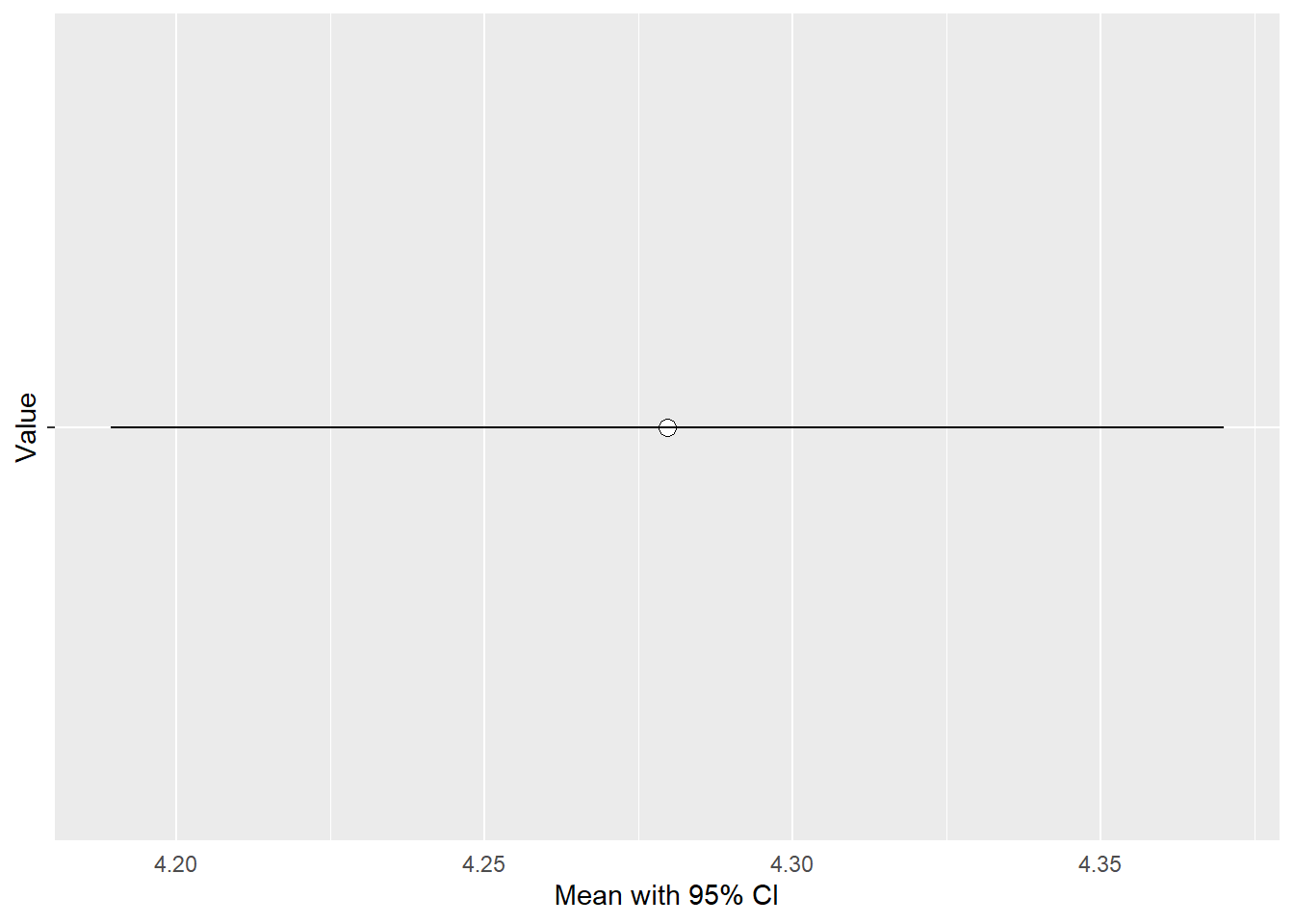
4.4.2.2 Proportion
Besides the mean, we can calculate a confidence interval for a proportion value of a sample. The formula is slightly different because the calculation of the standard error is different. It is the square root of the variance divided by the number of observations. The variance is obtained by multiplying the probability of an event \(p\) times the counter probability \(1-p\):
\(95\% CIs=[p - 1.96 \times \sqrt{\frac{p\times(1-p)}{n}}, p + 1.96 \times \sqrt{\frac{p\times(1-p)}{n}}]\).
Let’s try this by using a dichotomized version of the government satisfaction variable with an initial 11-point rating scale. In this example, values of 5 or less are assigned to 0 (“little or not satisfied”) and values above 5 are assigned to 1 (“satisfied”). We can now focus on the proportion of those respondents who are satisfied or rather satisfied with the government (variable value = 1). Note that with a 0/1 coding, the mean of a binary variable corresponds to the proportion of observations with a variable value of 1.
# Recode of variable
data_ess <- data_ess %>%
  mutate(stfgov_di =
           case_when(stfgov <= 5 ~ 0,
                     stfgov > 5 ~ 1))

# Proportion via table command
prop.table(table(data_ess$stfgov_di))
##
## 0 1
## 0.693281 0.306719
# Correspondence with the mean of the summary command
summary(data_ess$stfgov_di)
## Min. 1st Qu. Median Mean 3rd Qu. Max. NA's
## 0.0000 0.0000 0.0000 0.3067 1.0000 1.0000 66
# Set confidence level with 1-alpha
conf.level <- 0.95

# Calculating the critical z-value for a two-sided test
z <- qnorm((1 + conf.level) / 2)

# Calculation of the confidence interval
lower.ci <- 0.3067 - z * sqrt((0.3067*(1-0.3067))/n)
upper.ci <- 0.3067 + z * sqrt((0.3067*(1-0.3067))/n)

# Print the confidence intervals
cat("The", conf.level*100, "% confidence interval for the proportion value is (", round(lower.ci, 2), ",", round(upper.ci, 2), ").\n")
## The 95 % confidence interval for the proportion value is ( 0.29 , 0.33 ).
# Test using t.test
t.test(data_ess$stfgov_di, conf.level = 0.95)
##
## One Sample t-test
##
## data: data_ess$stfgov_di
## t = 31.837, df = 2291, p-value < 2.2e-16
## alternative hypothesis: true mean is not equal to 0
## 95 percent confidence interval:
## 0.2878265 0.3256115
## sample estimates:
## mean of x
## 0.306719Question: Interpret the confidence interval.
Your answer:
Solution:
Interpretation: Likely values for the population proportion are within the limits of 0.29 and 0.33.
4.4.2.3 Correlation coefficient
Next, we look at how a confidence interval for a correlation is computed. For this, we use the following formula: \(95\% CIs=r\pm 1.96 \times SE\), where the standard error SE is calculated as follows: \(SE_r=\sqrt {\frac{(1-r^2)}{n-2}}\). To illustrate that, we let the software compute the confidence interval of the correlation between household income and satisfaction with the government. hinctnta measures respondents’ net household income (after deductions) across 10 quantiles (“deciles” 1-10) - the reason for this measurement is that this way income becomes adjusted to a country’s income distribution and is thus comparable across countries. Regarding the correlation, we assume that - in line with economic voting theory - people with a higher income are more satisfied with the government than people with a lower income.
cor <- cor.test(data_ess$hinctnta, data_ess$stfgov)
cor
##
## Pearson's product-moment correlation
##
## data: data_ess$hinctnta and data_ess$stfgov
## t = 1.805, df = 2047, p-value = 0.07122
## alternative hypothesis: true correlation is not equal to 0
## 95 percent confidence interval:
## -0.003445968 0.083023781
## sample estimates:
## cor
## 0.03986354Question: Interpret the confidence interval.
Your answer:
Solution:
Interpretation: Likely values for correlation in the population are within the limits of -0.003 and 0.08.
The graphical representation of the confidence interval of a correlation is two-dimensional. The width of the confidence interval can vary along the values of the x-axis. The value from the previous test is, so to say, the average confidence interval.
ciplot <- ggplot(data=data_ess, aes(x = hinctnta , y = stfgov)) +
  geom_smooth(method = lm, se = TRUE, level = 0.95) +
  xlab("Income (Deciles)") +
  ylab("Satisfaction with the government")
ciplot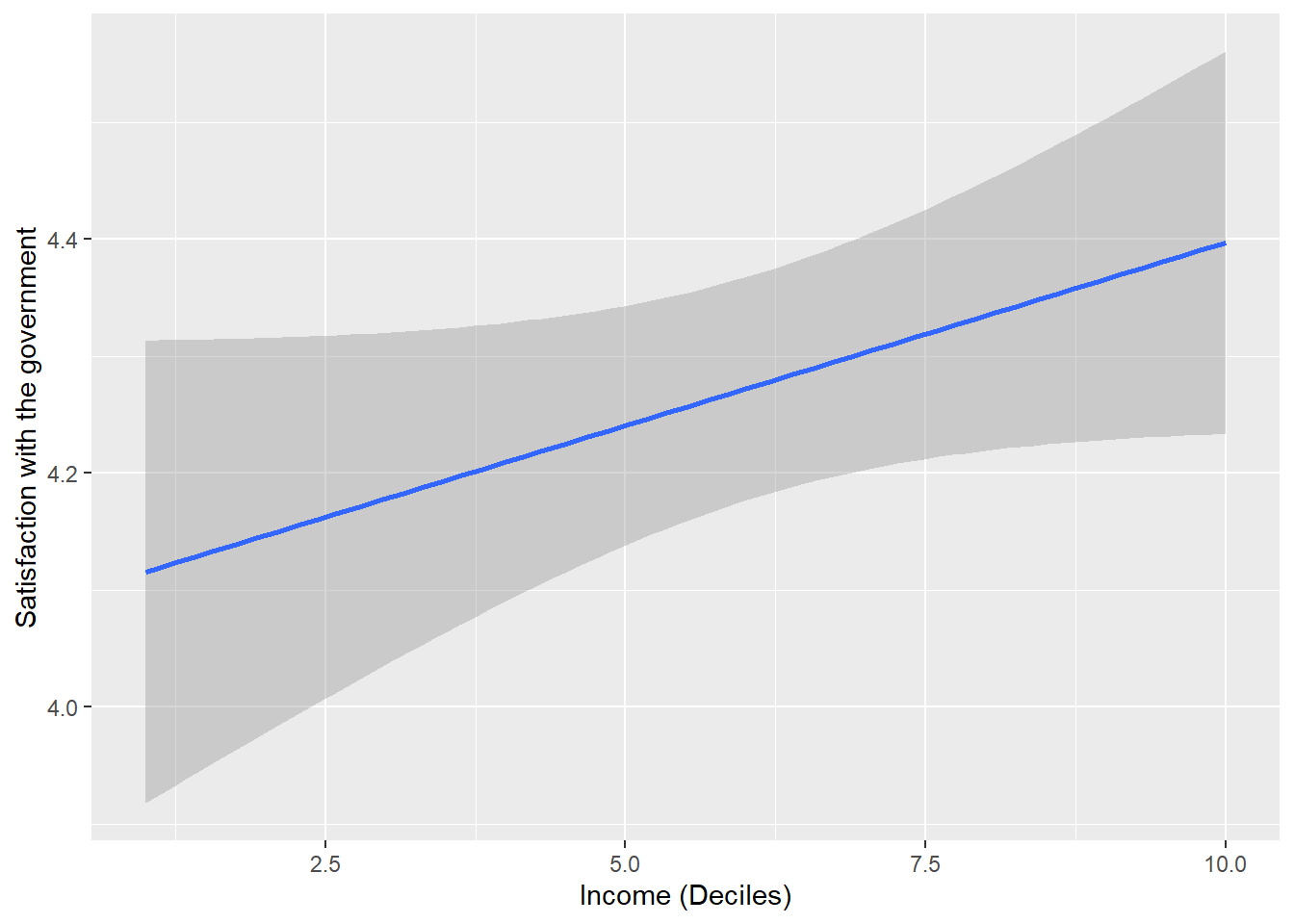
Question: The shown figure displays 95% confidence intervals. Would 90% confidence intervals be narrower or wider?
Your answer:
Solution:
The 90% confidence intervals would be narrower. Going back to the probability-world interpretation: If we only want to capture the true population parameter 90 percent of the time (instead of 95), this means that we could narrow down the range of values in which the parameter will fall. In contrast, if we decrease our readiness to err to 1% (i.e., a 99% confidence interval), the range of values to fulfill this assumption would increase - the confidence interval would get wider.
4.5 Null Hypothesis Testing
4.5.1 Basic idea and procedure
Hypothesis testing allows us to test how likely it is that a sample estimate corresponds to another value, more specifically the sampling distribution of another value. We typically use for this purpose the distribution that is obtained under the null hypothesis- that is, for example, the assumption that the difference in means between two groups or the correlation between two variables is zero in the population. The distribution of a test statistic under the assumption that the null hypothesis is true is sometimes labeled “null distribution.” We know from the central limit theorem that such a sampling distribution would be normal given repeated sampling and a high enough sample size (>30), which implies that we can use a normal distribution for our statistical tests.
The goal usually is to test the sample estimate we obtained against the null distribution. If the estimate is so “extreme” that it becomes very unlikely to obtain such a result although the null hypothesis is true, then this would provide evidence against the null hypothesis and in favor of our alternative hypothesis (e.g., the correlation between two variables is positive in the population). Hence, the procedure of Null Hypothesis Testing is a form of proof by contradiction. We assume the opposite of what we want to show and then collect as much evidence as possible against that assumption.
To begin with, we first formulate the so-called null hypothesis \(H_0\) (e.g., there is no or zero correlation in the population). Next, we formulate an alternative hypothesis \(H_A\) (e.g., the correlation in the population is positive or negative) and then want to show that the correlation we found is strong enough so that it becomes very unlikely that \(H_0\) is true. This means that we are trying to disprove \(H_0\), which in turn is evidence for \(H_A\). Note that we do not assign probabilities for \(H_A\) to be true but probabilities to observe a given estimate given that \(H_0\) is true (i.e., \(P\)(correlation | \(H_0\)).
The following steps illustrate how to do Null Hypothesis Testing:
- Step 1: Formulate the null hypothesis and alternative hypothesis.
- Step 2: Determine the probability of error (\(\alpha\), i.e., our willingness to err in repeated sampling, the convention is typically 5% or less).
- Step 3: Compute the value of the test statistic for your estimate (=estimator/standard error).
- Step 4a: Determine a critical value c (e.g., from an online table)
- Step 5a: If the value of the test statistic falls within the rejection range (i.e., exceeds the critical value), reject \(H_0\).
Alternatively:
Step 4b: Calculate p-value (use statistical software).
Step 5b: If p-value < probability of error, then reject \(H_0\).
Step 6: Interpret the result of the hypothesis test in substantive terms.
4.5.2 Hypothesis test of a difference in means
Differences in means usually refer to a comparison of the mean of a variable between two groups. To illustrate that, we use the example of income and government satisfaction again. We leave the variable government satisfaction stfgov in its original metric form so that we can calculate the mean. However, we dichotomize the variable income hinctnta into two groups: low earners and high earners.
data_ess <- data_ess %>%
  mutate(hinctnta_di =
           case_when(hinctnta <= 6 ~ 0,
                     hinctnta > 6 ~ 1))
summary(data_ess$hinctnta_di)
## Min. 1st Qu. Median Mean 3rd Qu. Max. NA's
## 0.0000 0.0000 0.0000 0.4794 1.0000 1.0000 270Question: Formulate the null and alternative hypotheses if we assume that persons with a high-income are more satisfied with the government.
Your answer:
Solution:
Typically, it is easier to start with formulating the alternative hypothesis.
\(H_A\): High-income individuals are more satisfied with government than low-income individuals (i.e., positive relationship between income and satisfaction with government).
Formal: \(\mu(satisfaction|highincome)>\mu(satisfaction|lowincome)\) or (equivalent) \(\mu(satisfaction|highincome)-\mu(satisfaction|lowincome)>0\)
\(H_0\): High-income individuals are equally or less satisfied with government than low-income individuals (i.e., null or negative relationship between income and satisfaction with government).
Formal: \(\mu(satisfaction|highincome)\le\mu(satisfaction|lowincome)\) or (equivalent) \(\mu(satisfaction|highincome)-\mu(satisfaction|lowincome)\le0\)
Note that it is important that all possible outcomes are covered by both hypotheses. This means that when formulating a directed hypothesis, the null hypothesis must include the case of no relationship (i.e., “\(\le\)” instead of just “\(<\)”).
Let us then assume an error probability of 5% or 0.05 (Step 2). Next, we calculate the test statistic (Step 3). Generally, this is given as \(\frac{estimate - true value}{standard error}\). Since we test against the null hypothesis, the true value is 0. The formula for the so-called z-test statistic is given as:
\(z=\frac{Estimation}{Standard Error}\).
Steps 4 and 5 are about the actual test. Remember that per the alternative hypothesis, we assumed a positive mean difference (i.e., high-income earners are more satisfied with the government than low-income earners). Next, we want to know where the mean difference is located on the null distribution. If it is close to the center of the distribution, we have no reason to reject the null hypothesis. However, if it is at the margins of the distribution, this would provide a reason for rejecting the null hypothesis (and favoring the alternative hypothesis). We use the z-distribution with a mean of 0 and a standard deviation of 1. Remember the properties of this distribution from above. If we set the critical value to be lower than -1.96 and higher than +1.96, we would be in the 5% range of the distribution if our test statistic exceeds those critical values. If this was the case, we can conclude that it would be very unlikely to sample such a value even though \(H_0\) holds. Note that we set up a positive and negative area of rejection if we formulate undirected hypotheses (i.e., \(H_A\): the mean difference can be higher or lower than zero, \(H_0\): the mean difference equals zero) and conduct two-sided tests. For a directed hypothesis (and one-sided tests), like in our example, the rejection area is only in the negative or positive range of the distribution (depending on whether \(H_A\) expects a pos. or neg. statistic).
# Draw a standard normal distribution:
z = seq(-4, 4, length.out=1001)
x = rnorm(z)

# Null distribution of two-sided test
plot( x=z, y=dnorm(z), bty='n', type='l', main="Null distribution of two-sided test, error probability 0.05", ylab="Probability density", xlab="z", xlim=c(-3,3))
axis(1, at = seq(-4, 4, by = 1))
polygon(x=c(z[z<=qnorm(0.025)], qnorm(0.025), min(z)), y=c(dnorm(z[z<=qnorm(0.025)]), 0, 0), col="maroon")
polygon(x=c(z[z>=qnorm(0.975)], max(z), qnorm(0.975)), y=c(dnorm(z[z>=qnorm(0.975)]), 0, 0), col="maroon")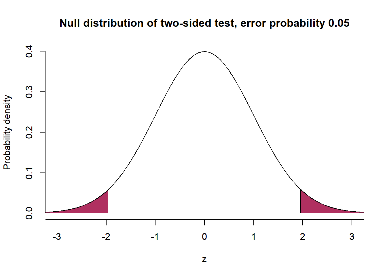
# Null distribution of one-sided test (H_A>0)
plot( x=z, y=dnorm(z), bty='n', type='l', main="Null distribution of one-sided test (H_A>0), error probability 0.05", ylab="Probability density", xlab="z", xlim=c(-3,3))
axis(1, at = seq(-4, 4, by = 1))
polygon(x=c(z[z>=qnorm(0.95)], max(z), qnorm(0.95)), y=c(dnorm(z[z>=qnorm(0.95)]), 0, 0), col="maroon")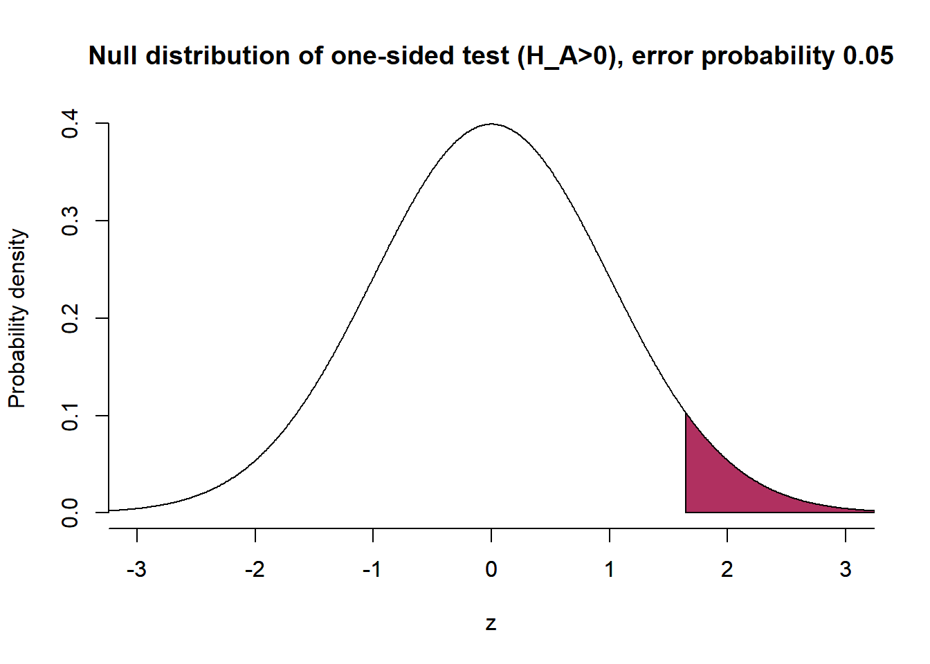
# Null distribution of one-sided test (H_A<0)
plot( x=z, y=dnorm(z), bty='n', type='l', main="Null distribution of one-sided test (H_A<0), error probability 0.05", ylab="Probability density", xlab="z", xlim=c(-3,3))
axis(1, at = seq(-4, 4, by = 1))
polygon(x=c(z[z<=qnorm(0.05)], qnorm(0.05), min(z)), y=c(dnorm(z[z<=qnorm(0.05)]), 0, 0), col="maroon")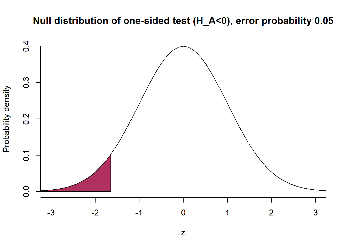
Question: How would the rejection area change if we test one-sided? What would change if we set a 1% probability of error (two-sided test)?
Your answer:
Solution:
Assuming a positive mean difference or correlation, the rejection area would be located only on the right side of the distribution. Since we still use an error probability of 5%, this area would be larger than in the two-sided case. Consequently, the critical value c thus moves a bit in the direction of the center of the distribution. For the z-distribution, this value is +1.645 for a positive alternative hypothesis (and -1.645 for a negative hypothesis).
If we change the probability of error to 1% and test two-sided, we have a rejection range that is smaller compared to the 5% case. Our estimate and the corresponding z-statistic need to be larger to reject the null hypothesis compared to the 5%-case. In the 1% case, the critical values are -2.326 and +2.326.
Critical values at which one can reject the null hypothesis can be obtained from here: https://www.criticalvaluecalculator.com/
4.5.2.1 General remarks on P-values
P-values indicate the probability of finding an estimate as extreme (or more extreme) as we got from our sample (e.g., a difference in means), even though the null hypothesis is true in the population. In formal terms, that is the probability of the estimate given the null hypothesis \(P\)(estimate | \(H_0\)).
Some features of p-values:
The smaller the p-value, the more “statistically significant” the result (or the more reason we have to reject the null hypothesis, which, in turn, provides evidence in favor of the alternative hypothesis).
Contingent upon the probability of error, if p is smaller than \(\alpha\), then the result is statistically significant (usually < 0.05 or 5%).
If the test statistic associated with the estimate is less than or greater than the critical z- or t-values, respectively, then p < 0.05.
-
Correspondence with confidence intervals:
If the confidence interval includes the null hypothesis value (usually 0), this is consistent with a high p-value, indicating weak evidence against the null hypothesis.
If the confidence interval does not include 0, it is consistent with a low p-value, suggesting strong evidence against the null hypothesis.
For example: A mean difference of 0.5 with a 95% confidence interval of [0.35; 0.65] is statistically significant at the \(\alpha\)=0.05 level (reject \(H_0\)). However, a mean difference of -0.1 with a 95% confidence interval of [-0.25; 0.05] is statistically not significant at the \(\alpha\)=0.05 level (confidence intervals include 0, fail to reject \(H_0\)).
To calculate the exact p-value, we rely on tables or statistical software.
A p-value says nothing about the probability that \(H_0\) or \(H_A\) is true; remember \(P\)(estimate | \(H_0\))!
When we formulate one-sided hypotheses but use a two-sided test (which is the norm in social science research), we are especially careful and do not want to make a 1st kind error (\(H_0\) is true, but we reject it); we can divide the p-value by 2 and end up with the p-value we would have gotten if we tested one-sided.
4.5.2.2 Test implementation
To actually test the difference in the means of satisfaction with the government between high and low earners, the formula for this is given as \(z =\frac{(\bar x_1 - \bar x_2)}{standard error}\) (note that the standard error of the mean difference is not simply the difference of two standard errors).
We now calculate the mean difference and conduct a corresponding hypothesis test:
mean(data_ess$stfgov[data_ess$hinctnta_di==1], na.rm = TRUE)-
  mean(data_ess$stfgov[data_ess$hinctnta_di==0], na.rm = TRUE)
## [1] 0.1543566
t.test(data_ess$stfgov[data_ess$hinctnta_di==1], data_ess$stfgov[data_ess$hinctnta_di==0])##
## Welch Two Sample t-test
##
## data: data_ess$stfgov[data_ess$hinctnta_di == 1] and data_ess$stfgov[data_ess$hinctnta_di == 0]
## t = 1.5882, df = 2046.8, p-value = 0.1124
## alternative hypothesis: true difference in means is not equal to 0
## 95 percent confidence interval:
## -0.03624397 0.34495717
## sample estimates:
## mean of x mean of y
## 4.354545 4.200189Question: Interpret the result of the statistical test in detail with reference to the specific p-value.
Your answer:
Solution:
The probability of obtaining such a result from the sample, although \(H_0\) is true in the population, is 0.11 or 11%. Since this exceeds the threshold of our willingness to err of 5%, we cannot reject the null hypothesis (and thus find no evidence in favor of \(H_A\)).
Even if we take into account that we formulated a directed hypothesis and rely on a one-sided test (we can thus divide the p-value by 2), the p-value still exceeds our assumed probability of error (p-value of 0.055 > \(\alpha\) of 0.05). Hence, even with a one-sided test, we are not able to reject the null hypothesis.
4.5.3 Hypothesis test of a correlation
Instead of a difference in means, we now focus on hypothesis tests of correlations. The procedure is analogous to the one before. We first formulate the null and alternative hypotheses, specify the probability of error (5% in this case), calculate the test statistic (\(z=\frac{r}{SE}\)), calculate the p-value, and interpret the result.
Question: Assume that higher income is either positively or negatively related to satisfaction with government. Formulate the null and alternative hypotheses (undirected).
Your answer:
Solution:
\(H_A\): Verbal: Income is either positively or negatively related to satisfaction with government.
Formal: \(r \ne 0\)
\(H_0\): Verbal: Income is unrelated to satisfaction with government.
Formal: \(r = 0\)
We now calculate the test statistic and the p-value.
cor <- cor.test(data_ess$hinctnta, data_ess$stfgov)
cor
##
## Pearson's product-moment correlation
##
## data: data_ess$hinctnta and data_ess$stfgov
## t = 1.805, df = 2047, p-value = 0.07122
## alternative hypothesis: true correlation is not equal to 0
## 95 percent confidence interval:
## -0.003445968 0.083023781
## sample estimates:
## cor
## 0.03986354Question: Interpret the result of the statistical test (two-sided test) with reference to the t-value and p-value.
Your answer:
Solution:
The probability of obtaining such a result from the sample, although \(H_0\) is true in the population, is 0.07 or 7%. Since this exceeds the threshold of our willingness to err of 5%, the result is not statistically significant and we cannot reject the null hypothesis (and thus find no evidence in favor of \(H_A\)).
4.6 Outlook
This case study reviewed the basics of probability theory, some relevant statistical laws, confidence intervals, and hypothesis testing. In the examples, we have mainly used the z-distribution, which is the way to go if we deal with large or reasonably large samples (>30 is already sufficient). For small samples and other purposes, we use other distributions for statistical testing that are briefly introduced here.
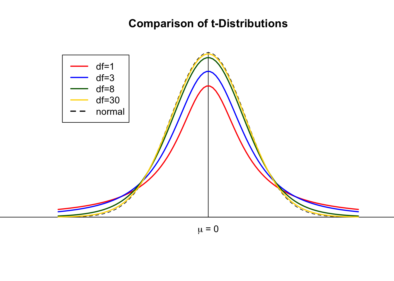
4.6.1 t-distribution
The t-distribution corresponds to the z-distribution for larger samples. For small samples, the distribution is flatter and therefore has wider margins. The critical t-values (above or below we can reject the null hypothesis) are therefore larger on the right and lower on the left side. This makes it more difficult to reject the null hypothesis. In other words: We need more extreme results in small samples to reject the null hypothesis. This accounts for the fact that some outliers have greater weight in small samples. This helps to avoid the so-called alpha error (or type I error), which refers to erroneously inferring statistically significant results although the null hypothesis is true in the population. The alpha error is usually seen as a greater threat to scientific progress than failing to reject the null hypothesis although we should have done so (beta error or type II error).
Df refers to degrees of freedom, which is usually the number of cases - 1 (for estimation).
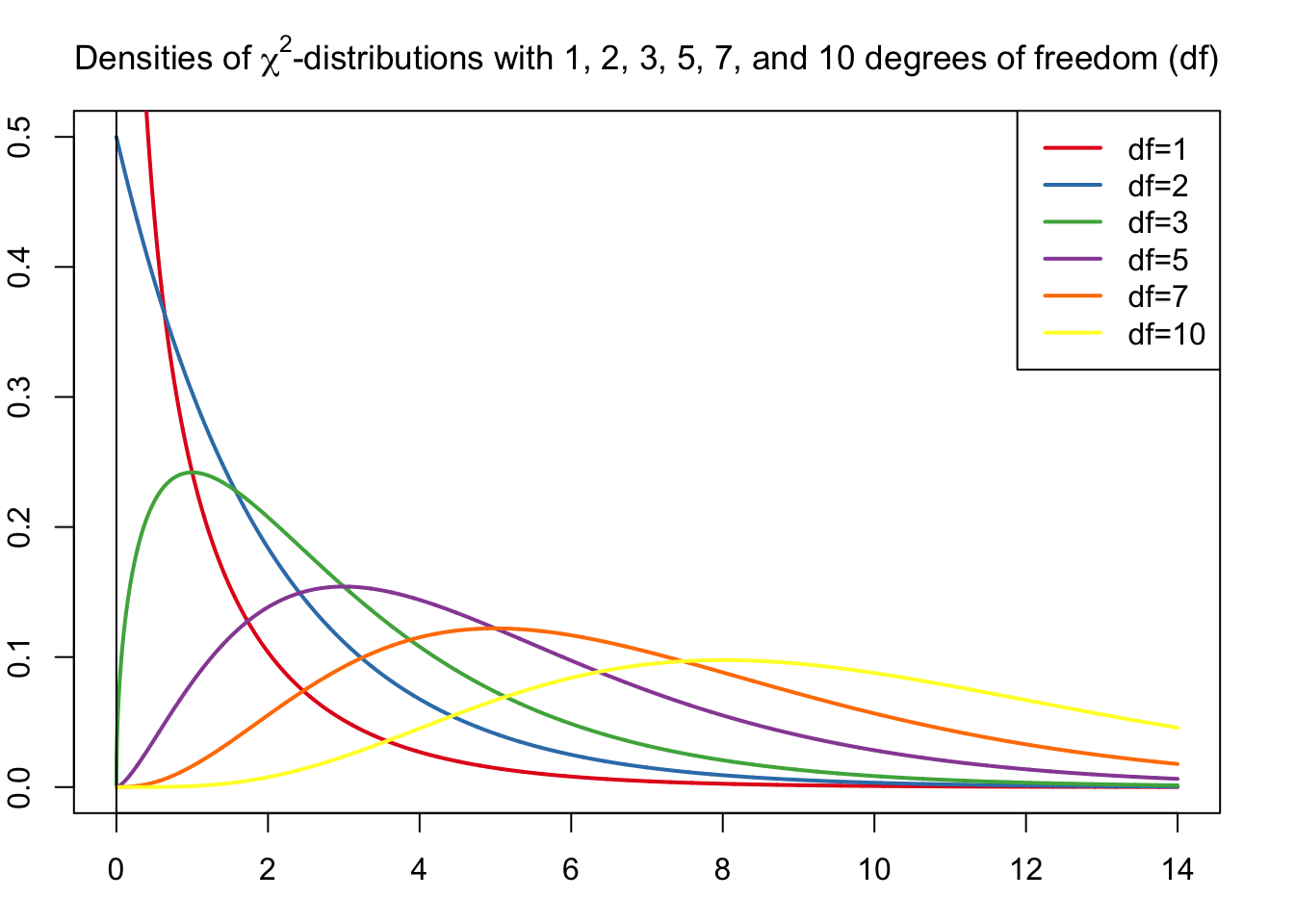
4.6.2 Chi-square distribution
The chi-square distribution is used, for example, for testing variances. One field of application is in cross tabulations. Chi-square values are never negative, so only one-sided tests are suitable.
Df refers to degrees of freedom, which in the case of crosstabs would be the table size, for example.
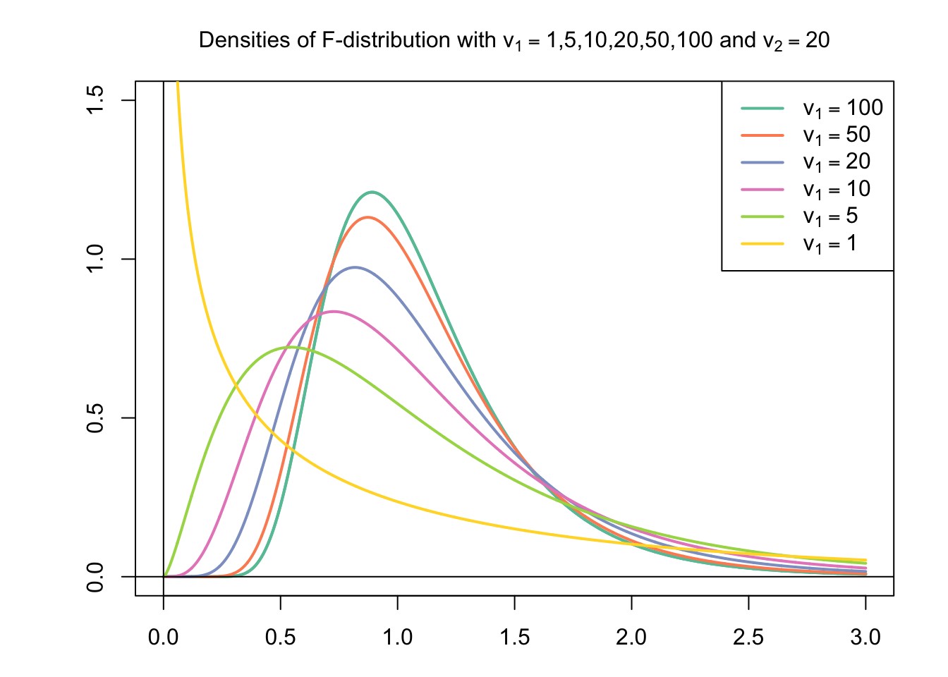
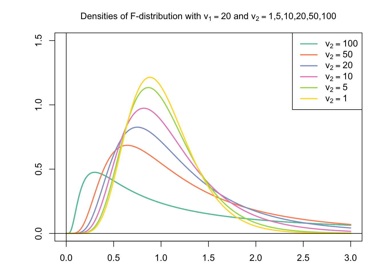
4.6.3 F-Distribution
The F-distribution is basically the ratio of two chi-squared distributed random variables (e.g., two variances). The F-distribution is also always positive and the functional form depends on the degrees of freedom of the two variables under consideration. F-tests are used, for example, in comparing the model fit of regression models.
4.6.4 Statistical versus substantive significance
The procedures discussed here relate to the concept of hypothesis testing and statistical significance. They are essentially concerned with quantifying uncertainty and inferring from that whether or not one can assume that a result from a random sample can be generalized to the population the sample has been drawn from. Although these are important concepts, statistical significance is different from scientific or substantive significance, which refers to the degree to which a result is relevant against the background of other research findings or alternative explanatory factors. Thus, a statistically significant result may not be substantial or, conversely, a substantial result may not be statistically significant. Statistical significance, for example, is highly dependent on the number of observations that are incorporated in calculating the standard error. A measure of the substance of, for example, a regression coefficient can be obtained by using standardized effect sizes such as beta or Cohen’s D.
In general, we are looking for empirical results that are both statistically and substantively significant.