5 Regression Analysis - Case Study Attitudes Toward Justice
In this case study, we use survey data from the 2021 German General Population Survey of the Social Sciences (German: ALLBUS). Specifically, we examine the relationship between income and attitudes toward social justice.
First, we prepare the data and analyze the bivariate relationship between income and attitudes toward social justice.
Second, we control for possible alternative explanations in a multiple regression model. Here we focus on the “confounding variables” gender of respondents and whether or not respondents have been unemployed in the past 10 years.
Third, we take a look at regression diagnostics, how to model nonlinear relationships between variables, and interactions between variables.
5.1 Data preparation and bivariate regression
First, we read the data set and get an overview of the variables in the data set.
data_allbus <- read_dta("data/allbus2021_reduziert.dta")

# Here all cases are deleted, which have missing values on any of the variables. This is only recommended for reduced data sets with few variables, otherwise you would "throw out" observations based on non-relevant variables
data_allbus <- na.omit(data_allbus)

# We also delete three observations that indicated "diverse" for the gender variable, as this simplifies hypothesis generation
data_allbus<-subset(data_allbus, sex!=3)

# We now recode variables
data_allbus$income <- data_allbus$incc

data_allbus <- data_allbus %>%
  mutate(female =
           case_when(sex == 1 ~ 0,
                     sex == 2 ~ 1))

data_allbus <- data_allbus %>%
  mutate(east =
           case_when(eastwest == 1 ~ 0,
                     eastwest == 2 ~ 1))

data_allbus <- data_allbus %>%
  mutate(unemployed =
           case_when(dw18 == 1 ~ 1,
                     dw18 == 2 ~ 0))

# Summarize and overview data
summary(data_allbus)
## eastwest sex im19 im20 im21
## Min. :1.000 Min. :1.000 Min. :1.000 Min. :1.00 Min. :1.000
## 1st Qu.:1.000 1st Qu.:1.000 1st Qu.:2.000 1st Qu.:2.00 1st Qu.:2.000
## Median :1.000 Median :1.000 Median :3.000 Median :3.00 Median :3.000
## Mean :1.308 Mean :1.486 Mean :2.771 Mean :2.82 Mean :2.984
## 3rd Qu.:2.000 3rd Qu.:2.000 3rd Qu.:3.000 3rd Qu.:3.00 3rd Qu.:4.000
## Max. :2.000 Max. :2.000 Max. :4.000 Max. :4.00 Max. :4.000
## dw18 incc income female
## Min. :1.000 Min. : 1.0 Min. : 1.0 Min. :0.0000
## 1st Qu.:2.000 1st Qu.:13.0 1st Qu.:13.0 1st Qu.:0.0000
## Median :2.000 Median :15.0 Median :15.0 Median :0.0000
## Mean :1.812 Mean :15.3 Mean :15.3 Mean :0.4859
## 3rd Qu.:2.000 3rd Qu.:19.0 3rd Qu.:19.0 3rd Qu.:1.0000
## Max. :2.000 Max. :26.0 Max. :26.0 Max. :1.0000
## east unemployed
## Min. :0.0000 Min. :0.0000
## 1st Qu.:0.0000 1st Qu.:0.0000
## Median :0.0000 Median :0.0000
## Mean :0.3079 Mean :0.1884
## 3rd Qu.:1.0000 3rd Qu.:0.0000
## Max. :1.0000 Max. :1.0000
kable(head(data_allbus, 10), format = "html", booktabs = TRUE, caption = "ALLBUS survey data") %>%
    kable_paper() %>% #Font scheme of the table
scroll_box(width = "100%", height = "100%") #Scrollable box| eastwest | sex | im19 | im20 | im21 | dw18 | incc | income | female | east | unemployed |
|---|---|---|---|---|---|---|---|---|---|---|
| 1 | 2 | 4 | 3 | 4 | 2 | 9 | 9 | 1 | 0 | 0 |
| 1 | 1 | 4 | 4 | 4 | 2 | 17 | 17 | 0 | 0 | 0 |
| 1 | 2 | 2 | 3 | 4 | 2 | 7 | 7 | 1 | 0 | 0 |
| 1 | 2 | 4 | 4 | 3 | 2 | 21 | 21 | 1 | 0 | 0 |
| 1 | 1 | 2 | 3 | 3 | 2 | 21 | 21 | 0 | 0 | 0 |
| 1 | 2 | 2 | 3 | 3 | 2 | 4 | 4 | 1 | 0 | 0 |
| 1 | 2 | 2 | 2 | 3 | 2 | 13 | 13 | 1 | 0 | 0 |
| 1 | 1 | 4 | 4 | 3 | 2 | 20 | 20 | 0 | 0 | 0 |
| 1 | 1 | 1 | 2 | 3 | 2 | 17 | 17 | 0 | 0 | 0 |
| 1 | 2 | 2 | 3 | 3 | 2 | 7 | 7 | 1 | 0 | 0 |
Next, we build an index from the variables im19 (agreement: income differences increase motivation), im20 (agreement: rank differences between people are acceptable) and im21 (agreement: social differences are fair). Since high values on those variables indicate disagreement, we can label the index morejustice for which high values represent disagreement with social inequality (i.e., advocacy of more justice).
Your answer:
Solution:
Yes, if we were to recode all items, that would be just as possible. We would then have to label an index as “less justice” or “inequality,” since high values represent acceptance of social inequality. Recoding only a few variables is inadmissible, the index would no longer be valid.
For building scales or indices of items, it is always a good idea to check whether there are substantial correlations between the items. There are also other ways to look at the reliability of an index, for example, by calculating Cronbach’s alpha. We go with correlations and also look at the distribution of the index variable.
# Do the items correlate sufficiently high for the index? (>.4 would be desirable)
# Calculate correlation and output
vars <- c("im19", "im20", "im21")
cor.vars <- data_allbus[vars]
rcorr(as.matrix(cor.vars))
## im19 im20 im21
## im19 1.00 0.46 0.33
## im20 0.46 1.00 0.51
## im21 0.33 0.51 1.00
##
## n= 2595
##
##
## P
## im19 im20 im21
## im19 0 0
## im20 0 0
## im21 0 0
# Index creation
data_allbus$morejustice <- (data_allbus$im19 + data_allbus$im20 + data_allbus$im21)/3
hist(data_allbus$morejustice)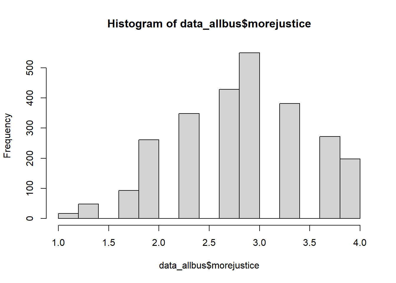
The correlations show that at least most of the indicators are correlated with each other by r > .4. The histogram suggests that the variable values are approximately normally distributed.
5.1.1 The foundations of (bivariate) regression
In the next step, we will work our way into bivariate regression analysis. In order to calculate the relationship between two variables, a so-called slope line is calculated using the least squares method. The following figure shows the basic idea. These are fictitious data points.
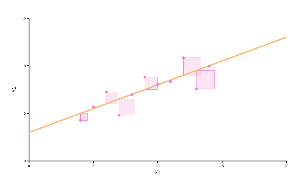 Source: https://seeing-theory.brown.edu/regression-analysis/index.html
Basically, this method allows us to find a straight line that optimally travels through the dots of observations. The smaller the squares, the better the line fits the data. We have found the optimal solution if any different slope of the line would lead to an increase in the sum of squared deviations. Hence, this estimator is called ordinary least squares - the OLS estimator. If we had more than one variable in the regression model, another spatial dimension would be added (a z-axis) and the straight line would become a surface. With more than two independent variables, we are dealing with a multidimensional surface that is no longer depictable. The least squares method remains the same in such a case, except that the computation becomes more complex (done with a software algorithm).
The software program computes a so-called regression coefficient for each independent variable (e.g., \(\beta_1\) for the corresponding variable \(X_1\)). In the bivariate case (one independent variable), the regression coefficient represents the “steepness” of the slope in the following way:
If \(X_1\) increases by one unit, then \(Y\) increases or decreases by \(\beta_1\) units (depending on the sign).
Let us now briefly remember the example from case study on univariate statistics, where we focused in the outlook on the empirical relationship between unemployment and crime rates in German counties. There we found a positive bivariate relationship between the two variables. The table below shows the coefficient estimate and the figure that depicts the positive association. If unemployment increases by one unit (here: 1 percentage point), then crime rates increase by 517.46 units (here: cases per 100T inhabitants), on average.
data_nrw <- read_excel("data/inkar_nrw.xls")
model1 <- lm(crimerate ~ 1 + unemp, data = data_nrw)
stargazer(model1, type = "text")
##
## ===============================================
## Dependent variable:
## ---------------------------
## crimerate
## -----------------------------------------------
## unemp 517.460***
## (69.412)
##
## Constant 2,398.594***
## (543.248)
##
## -----------------------------------------------
## Observations 53
## R2 0.521
## Adjusted R2 0.512
## Residual Std. Error 1,240.129 (df = 51)
## F Statistic 55.575*** (df = 1; 51)
## ===============================================
## Note: *p<0.1; **p<0.05; ***p<0.01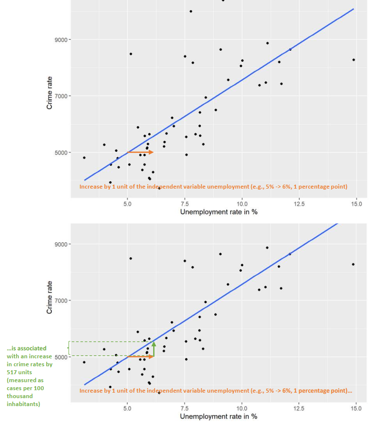
We can also think about what would happen if the dots (i.e., the observed values on the two variables) were different. If the dots and the corresponding slope line were steeper (and thus the coefficient larger), then an increase in unemployment by one unit would lead to an even higher increase in crime rates. If the dots and the line indicated a flat pattern, then this would mean that there is no change in crime rates when unemployment increases by one unit. If the line (and the coefficient) was negative, then a one-unit increase in unemployment would be associated with a decrease (by \(\beta_1\) units) in crime.
In addition to the coefficients for the independent variables, the regression output displays the so-called constant (or intercept), which is abbreviated as \(a\), \(\alpha\), or \(\beta_0\). It provides the predicted value for the outcome variable \(Y\) if all independent variables in the model have the value of 0. Usually, this information is not of much interest and thus ignored.
Your answer:
Solution:
The value of the constant in Model 1 is 2399. This indicates the average crime rate (Y) in a municipality with 0% unemployment. In our case, the constant is uninformative because we don’t have observations with 0% unemployment in our sample.
5.1.2 Bivariate regression of income and attitudes toward justice
We now estimate a bivariate regression for the relationship between income and attitudes toward justice. Our working hypothesis \(H_A\) is that we assume a negative relationship - that is, individuals with a higher income advocate less strongly social justice compared to individuals with a lower income (e.g., because they fear a loss of income due to redistributive policies).
Formally, \(H_A\) can be represented with reference to either a correlation coefficient \(r<0\) or a regression coefficient \(\beta_1<0\). Accordingly, the null hypothesis would be \(\beta_1\geq0\).
Your answer:
Solution:
Yes: For example, the higher the income, the higher the preference for social justice (since wealthier people can afford it). Which hypothesis makes sense depends on theory and previous research.
In a next step, the bivariate regression model is estimated. To do so, we use the index morejustice as the outcome and the variable income as an independent variable (or predictor), which measures income classes in 26 levels (e.g., 1 = under 200 EUR monthly net income; 14 = 1750 - 1999 EUR; 26 = 10000 EUR and more).
model_biv <- lm(morejustice ~ 1 + income, data = data_allbus) # 1 refers to the constant or intercept
summary(model_biv)
##
## Call:
## lm(formula = morejustice ~ 1 + income, data = data_allbus)
##
## Residuals:
## Min 1Q Median 3Q Max
## -2.12251 -0.49371 0.06216 0.46936 1.33916
##
## Coefficients:
## Estimate Std. Error t value Pr(>|t|)
## (Intercept) 3.140981 0.045227 69.449 < 2e-16 ***
## income -0.018467 0.002833 -6.518 8.53e-11 ***
## ---
## Signif. codes: 0 '***' 0.001 '**' 0.01 '*' 0.05 '.' 0.1 ' ' 1
##
## Residual standard error: 0.6574 on 2593 degrees of freedom
## Multiple R-squared: 0.01612, Adjusted R-squared: 0.01574
## F-statistic: 42.48 on 1 and 2593 DF, p-value: 8.532e-11
stargazer(model_biv, type = "text")##
## ===============================================
## Dependent variable:
## ---------------------------
## morejustice
## -----------------------------------------------
## income -0.018***
## (0.003)
##
## Constant 3.141***
## (0.045)
##
## -----------------------------------------------
## Observations 2,595
## R2 0.016
## Adjusted R2 0.016
## Residual Std. Error 0.657 (df = 2593)
## F Statistic 42.484*** (df = 1; 2593)
## ===============================================
## Note: *p<0.1; **p<0.05; ***p<0.01Task: Interpret the output from the regression model using the following heuristics.
“The empirical relationship between income and attitudes toward justice is positive/negative.”
“The relationship is/is not statistically significant.”
Use the technically correct interpretation of p-values: “The probability of finding such a relationship in the population, …”
“Thus, the null hypothesis can be rejected/not be rejected.”
The detailed interpretation of the regression coefficient for income is: “…”
Interpret additionally the constant and R2 from the model output. What is the value of the constant in the unemployment-crime example (Model 1)? What information content does it carry?Your answer:
Solution:
The empirical relationship between income and attitudes toward justice is negative.
The found relationship is statistically significant (given a probability of error of 0.01 or 1% due to ***).
The probability of finding such a relationship in the population, even though the null hypothesis is true, is less than 1%. Thus, the null hypothesis can be rejected.
The detailed interpretation of the regression coefficient for income (b=-0.018) is as follows: If income increases by one unit (income category), then (variant 1:) attitudes toward justice decrease (on average) by 0.018 units (scale points) / (variant 2:) changes by -0.018 units.
Constant: An interpretation is tedious because the income variable we used has no zero point. (If we would center the income variable at the mean value, then 0 indicated an average income, and the constant was the predicted level of justice attitudes for individuals with an average income.)
R2 is a measure of model fit and indicates how well the included independent variables explain the outcome. It can be interpreted as the ratio of explained variance by the model to the total variance: R2=0.016 -> 1.6% of the total variance of the outcome variable can be explained by the predictor variables in the model. If R2 = 0.3, then the variance explained by the model would be 30%.
Note: The so-called adjusted R2 is used to compare models with a different number of predictor variables. While it can no longer be interpreted as % of variance explained, it can be compared across models (better model with higher Adj-R2).5.1.3 On the correspondence of correlation coefficient and standardized regression coefficient in the bivariate case
Pearson’s correlation coefficient is the standardized covariance between two variables and corresponds to the so-called standardized regression coefficient from bivariate regression. To obtain the standardized regression coefficient, we can either z-transform the variables (\(z=\frac{(x-\bar{x})}{S_x}\)) before they enter the regression model or transform the coefficient after estimation by multiplying the unstandardized regression coefficient by the standard deviation of \(X\) and dividing the result by the standard deviation of \(Y\): \(\beta_s=\frac{(\beta*S_y)}{S_x}\).
In the present case, we obtain the standard deviations and then calculate the standardized coefficient by hand, as well as use the scale function in R that automatically z-transforms variables and then estimates the regression model. We will check whether both procedures and the correlation correspond to each other.
# Standardized regression coefficient by hand
sdx <- sd(data_allbus$income)
sdy <- sd(data_allbus$morejustice)

beta_s <- (-0.018281*sdx)/sdy
beta_s
## [1] -0.1256859
# Standardized regression coefficient with model
model_biv_s <- lm(scale(morejustice) ~ 1 + scale(income), data = data_allbus)
summary(model_biv_s)
##
## Call:
## lm(formula = scale(morejustice) ~ 1 + scale(income), data = data_allbus)
##
## Residuals:
## Min 1Q Median 3Q Max
## -3.2030 -0.7450 0.0938 0.7083 2.0209
##
## Coefficients:
## Estimate Std. Error t value Pr(>|t|)
## (Intercept) 2.553e-17 1.948e-02 0.000 1
## scale(income) -1.270e-01 1.948e-02 -6.518 8.53e-11 ***
## ---
## Signif. codes: 0 '***' 0.001 '**' 0.01 '*' 0.05 '.' 0.1 ' ' 1
##
## Residual standard error: 0.9921 on 2593 degrees of freedom
## Multiple R-squared: 0.01612, Adjusted R-squared: 0.01574
## F-statistic: 42.48 on 1 and 2593 DF, p-value: 8.532e-11
# Calculate correlation
vars <- c("income", "morejustice")
cor.vars <- data_allbus[vars]
rcorr(as.matrix(cor.vars))
## income morejustice
## income 1.00 -0.13
## morejustice -0.13 1.00
##
## n= 2595
##
##
## P
## income morejustice
## income 0
## morejustice 0Interpret the standardized regression coefficient as follows: If \(X\) (income) increases by one standard deviation, then Y increases/decreases by \(\beta_s\)-standard deviations. Here, it is a decrease by 0.13 standard deviations.
Standardized regression coefficients are also widely used in multiple regression (i.e., regressions with more than one independent variable). The advantage is that we “free” the variables from their original scale of measurement and use “standard deviations” as a comparable scale of measurement. We can thus directly compare regression coefficients. If a coefficient is larger, then it also has a larger “effect” on the outcome variable. For example, an increase of one unit on a scale of income that is measured on a scale ranging between 0 and 10,000 would result in a smaller change in the outcome variable than if it was measured on a scale with only 12 categories. Using standardized versions of each variable and using these two versions in two separate regression models should lead to comparable results. As an example of competing explanations that are represented by two independent variables in the same model: If income has a standardized coefficient of -0.13 and age has a standardized coefficient of -0.05, then income has a “greater effect” (on the outcome variable) than age.
Note that we typically report z-standardized coefficients only for metric (but not binary) predictor variables and that there are other routines for comparing coefficients, such as the min-max normalization where all variables have a minimum of 0 and a maximum of 1 (and ordinal or metric variables additional values in between 0 and 1).
5.2 Multiple Regression
5.2.1 Basic Idea
The goal of multiple regression is to explain the outcome variable with multiple independent variables. This is useful when we want to test different explanations for a phenomenon (e.g., attitudes toward justice). The multiple regression model produces adjusted estimates because the independent variables control for their mutual influences. Recall the example of unemployment and crime from the first case study, where we also included population density as an additional variable. The interpretation of the influence of unemployment (on crime) is in this case adjusted for the influence of population density. For unemployment, we obtained a coefficient estimate of \(\beta_1=215.4\). As a thought experiment: If we think of municipalities with the same population density and compare them with each other, then the municipalities with one percentage point more unemployment have on average a 215 higher crime rate per 100T inhabitants. The influence of population density on crime can be interpreted in a corresponding way - also here, the influence of the other factor (unemployment) is “held constant” or is controlled for.
This mutual “holding constant” or “controlling” in the multiple regression model means that we can account for alternative explanations with additional variables. In the example of attitudes toward justice, we use the variables gender (female with the categories male = 0 and female = 1), whether or not respondents were unemployed in the last 10 years (unemployed with the categories not unemployed = 0 and been unemployed = 1), and whether respondents live in West or East Germany (east with the categories West Germany = 0 and East Germany = 1) as additional variables. Regarding the influence of gender, we would assume that women are more supportive of social justice than men due to their socialization and societal norms and/or because they earn less than men, on average, due to the gender pay gap. Hence, it is important to control for gender so that income does not partially “transport” a gender effect. Controlling for gender in the multiple regression model allows us to obtain a “net” income effect that is separated from the effect of gender that otherwise could confound the relationship between income and attitudes toward justice.
Question: How relate past or current unemployment and living in East Germany to both variables of interest income and attitudes toward justice?
Your answer:
Solution:
Unemployment: If someone was/is unemployed, he/she is expected to advocate social justice more strongly (e.g. due to self-interest) than someone lacking such an experience. If someone is unemployed, he/she has a lower income, on average, compared to someone who is employed.
East Germany: East Germans are expected to advocate social justice more strongly than West Germans because of a greater sense of disadvantage or their socialization in the socialist GDR. At the same time, residents of East Germany have a higher probability to earn less money in comparable jobs due to a less developed economic situation.
5.2.2 Formulating hypotheses
The multiple regression model with four independent variables can be represented with the following formula:
\(y = \beta_0 + \beta_1 * x_1 + \beta_2 * x_2 + \beta_3 * x_3 + \beta_4 * x_4 + e\)
Y refers to the outcome variable, \(\beta_0\) is the constant, the other \(\beta_i\) are the regression coefficients of the corresponding predictor variables \(x_i\). \(e\) refers to the residual or the part of the variance of the outcome variable that is not explained by the predictor variables in the model.
If we use the variable names for this, the formula for the specific model would be the following:
\(morejustice = \beta_0 + \beta_1 * income + \beta_2 * female + \beta_3 * unemployed + \beta_4 * east + e\)
Question: Formulate the null and alternative hypotheses for each independent variable.
Your answer:
Solution:
Income
\(H_A\): \(\beta_1<0\) (Income is negatively related to attitudes toward justice)
\(H_0\): \(\beta_1\geq0\) (Income is unrelated or positively related to attitudes toward justice)
Female \(H_A\): \(\beta_2>0\) (Being female is positively related to attitudes toward justice, which is the same as women advocate social justice more strongly than men)
\(H_0\): \(\beta_2\leq0\) (Being female is unrelated or negatively related to attitudes toward justice)
Unemployed \(H_A\): \(\beta_3>0\) (Unemployment is positively related to attitudes toward justice, which is the same as people who experienced unemployment advocate social justice more strongly than those without such an experience)
\(H_0\): \(\beta_3\leq0\) (Unemployment is unrelated or negatively related to attitudes toward justice)
East Germany \(H_A\): \(\beta_4>0\) (Living in East Germany is positively related to attitudes toward justice, which is the same as people from East Germany advocate social justice more strongly than those from West Germany)
\(H_0\): \(\beta_4\leq0\) (Living in East Germany is unrelated or negatively related to attitudes toward justice)5.2.3 Estimation and result interpretation
We now estimate the corresponding regression model. The bivariate model has already been estimated above and is included for comparison.
model_mult <- lm(morejustice ~ 1 + income + female + unemployed + east, data = data_allbus)

stargazer(model_biv, model_mult, type = "text")
##
## =====================================================================
## Dependent variable:
## -------------------------------------------------
## morejustice
## (1) (2)
## ---------------------------------------------------------------------
## income -0.018*** -0.011***
## (0.003) (0.003)
##
## female 0.128***
## (0.028)
##
## unemployed 0.066**
## (0.033)
##
## east 0.075***
## (0.028)
##
## Constant 3.141*** 2.936***
## (0.045) (0.059)
##
## ---------------------------------------------------------------------
## Observations 2,595 2,595
## R2 0.016 0.027
## Adjusted R2 0.016 0.026
## Residual Std. Error 0.657 (df = 2593) 0.654 (df = 2590)
## F Statistic 42.484*** (df = 1; 2593) 18.263*** (df = 4; 2590)
## =====================================================================
## Note: *p<0.1; **p<0.05; ***p<0.01We can now insert the regression coefficients into the two formulas from above:
General form: \(y = 2.936-0.011 * x_1 + 0.128 * x_2 + 0.066 * x_3 + 0.075 * x_4 + e\)
Specific form: \(morejustice = 2.936-0.011 * income + 0.128 * female + 0.066 * unemployed + 0.075 * east + e\)
Question: Interpret the coefficients from the multiple regression model in terms of (a) direction of association, (b) significance, and (c) effect size.
Your answer:
Solution:
Negative relationship between income and attitudes toward justice, which is statistically significant (p < 0.01). An increase in income by one unit is associated with a decrease in attitudes toward justice by 0.011 scale units (while keeping the influence of the other variables in the model constant). In terms of effect size, moving from the lowest to the highest income category would be associated with a decrease in attitudes toward justice by 0.286 scale units (26 categories * 0.011 for the coefficient = 0.286, which corresponds to the effect of a min-max normalized income variable).
Positive relationship between being female and attitudes toward justice, which is statistically significant (p < 0.05). An increase in the variable female by one unit (= the difference between women and men) is associated with an increase in attitudes toward justice by 0.128 scale units (while keeping the influence of the other variables in the model constant).
Positive relationship between being unemployed in the last 10 years and attitudes toward justice, which is statistically significant (p < 0.05). An increase in the variable unemployment by one unit (= the difference between those who were unemployed and those who were not) is associated with an increase in attitudes toward justice by 0.066 scale units (while keeping the influence of the other variables in the model constant).
Positive relationship between living in East Germany and attitudes toward justice, which is statistically significant (p < 0.05). An increase in the variable east by one unit (= the difference between people from East vs. West Germany) is associated with an increase in attitudes toward justice by 0.075 scale units (while keeping the influence of the other variables in the model constant).
In terms of effect comparison, the variables female, unemployed, and east are measured on a comparable scale (0/1). The min-max effect of income is also comparable as this corresponds to recoding the variable to range between 0 and 1. Hence, income is comparatively the strongest predictor in the multiple regression model.
Question: What changed between the bivariate and the multiple model?
Your answer:
Solution:
In the multiple model (compared to the bivariate model), the coefficient of income (or the relationship between income and attitudes toward justice) is smaller. The underlying reason is that in the bivariate model, the coefficient partly represented unobserved factors, which is corrected in the multiple regression model (at least with respect to the variables included in the model).
5.3 OLS assumptions and model diagnostics, non-linear relationships between variables, and interactions
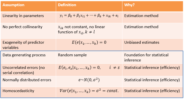
5.3.1 OLS assumptions
To obtain unbiased and efficient coefficient estimates from OLS regression models, several assumptions must be met. These assumptions refer to three areas.
- The first area ensures that the estimation method works at all. The first assumption is that the coefficients are additive because otherwise, the coefficients would not be estimable by the least squares method. This assumption is trivial and usually holds. Note that some statistic books erroneously cite this assumption that the empirical relationship between the independent and dependent variables must be linear. This is not the case and multiple linear regression can easily address non-linear relationships by multiplying variables with each other (see also below). The second assumption relates to the collinearity of independent variables. This means that two independent variables must not be perfectly correlated. Otherwise, the influence of one variable would be completely displaced by the influence of the other variable, which inhibits the reliable estimation of coefficients. It is rather rare that variables are too highly correlated with each other, and if there are variables in the dataset that measure similar constructs (and are thus highly correlated), one would build an index from those variables, anyway.
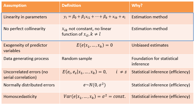
- The second area concerns the unbiasedness of coefficient estimates. The underlying assumption is exogeneity of independent variables. If a variable is exogenous, this ensures that the coefficient of this variable reflects the actual relationship and does not represent something else. This is defined as the error term (i.e., the variance of the outcome left unexplained which represents possible unobserved factors that yield an influence on the outcome) is unrelated to the predictor variables. In a randomized experiment, the treatment variable is an exogenous predictor (per design due to the randomization) that is unrelated to unobserved third variables. In a model with observational data (e.g., from a survey), the exogeneity assumption requires the exclusion of alternative explanations by including relevant control variables. If we have all relevant control variables in the model, this assumption would be met. However, if there are unobserved variables that are correlated with the predictor and the outcome variable (which is the rule rather than the exception), we have a problem: the exogeneity assumption is not met and the regression coefficient is biased. We cannot empirically determine the extent of this bias: There are no diagnostic tests for this assumption. This means that we need to do good theory work to get clarity about causal relationships between variables and to include relevant control variables in the regression model. Another way to go is - as already mentioned - using experimental designs to rule out alternative explanations.
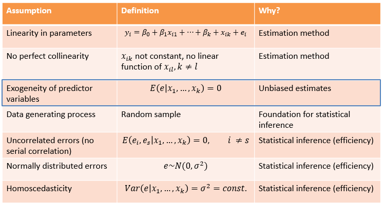
- The third area refers to the process of statistical inference. If the assumptions are violated, the standard errors and thus the test statistics (e.g., t/z statistics), and significance tests are biased. The unbiasedness of the coefficients (as in 2.) operates independently of this. The first assumption in this area relates to whether we work with a random sample. Without one, there is no basis for inferential statistics, although in practice inferential statistics are done even without a random sample. (Here one uses, for example, significance tests as information about how “reliable” or precise an empirical relationship is estimated.)
The assumption of uncorrelated errors means that each observation must carry a unique piece of information, independent of the information content of other observations in the sample. If we use, for example, cross-national survey data from different countries, observations within countries are possibly similar to each other regarding the outcome variable. For panel data, where the same units are observed multiple times over time, the similarity between observations from the same units is labeled serial correlation. If such a similarity between observations is not addressed by specific modeling choices (e.g., using multilevel models) or the variables included in the regression model, standard errors are biased. There are formal tests of uncorrelated errors, such as the Durbin-Watson Test.
The assumption that the errors must be normally distributed often serves as a rationale for assessing the distribution of variable values using a histogram and, if necessary, for transforming a variable so that its distribution is more “normal” (e.g., logarithmitize a right-skewed variable). This can be a useful strategy. At the same time, it is important to note that essentially the assumption refers to the distribution of errors (i.e., the outcome after accounting for variables in the model) and that with a sufficiently large number of observations, a violation becomes less problematic in terms of biased standard errors.
Finally, the assumption of homoscedastic standard errors states that the distribution of errors must be the same (or constant) for different values of the independent variable(s). If the assumption is violated and heteroscedasticity is present, then the standard errors are biased. Typically (but by no means always), there is an underestimation of the standard errors, which in turn is associated with overly optimistic significance tests (and type I errors). That is, we find a statistically significant result (and reject the null hypothesis) even though it is not actually a significant result. As a remedy, so-called robust standard errors can be applied.
5.3.2 Model diagnostics
5.3.2.1 Collinearity between variables -> VIF
To illustrate how to employ several existing tests of OLS assumptions, we use the above-estimated model model_mult.
The variance inflation factor (VIF) provides information on whether variables in the model are excessively correlated with other variables (this would also be registered in a correlation matrix of the variables, and one should be cautious if variables correlate with each other by more than 0.85). Regarding the VIF, a VIF above 5 is already a bit suspicious and a value above 10 indicates strong collinearity.
##Regression diagnostics
vif(model_mult)
## income female unemployed east
## 1.215933 1.175482 1.037561 1.014182The VIF is modest (< 5) for all variables in the model. We can conclude that there is no multicollinearity present.
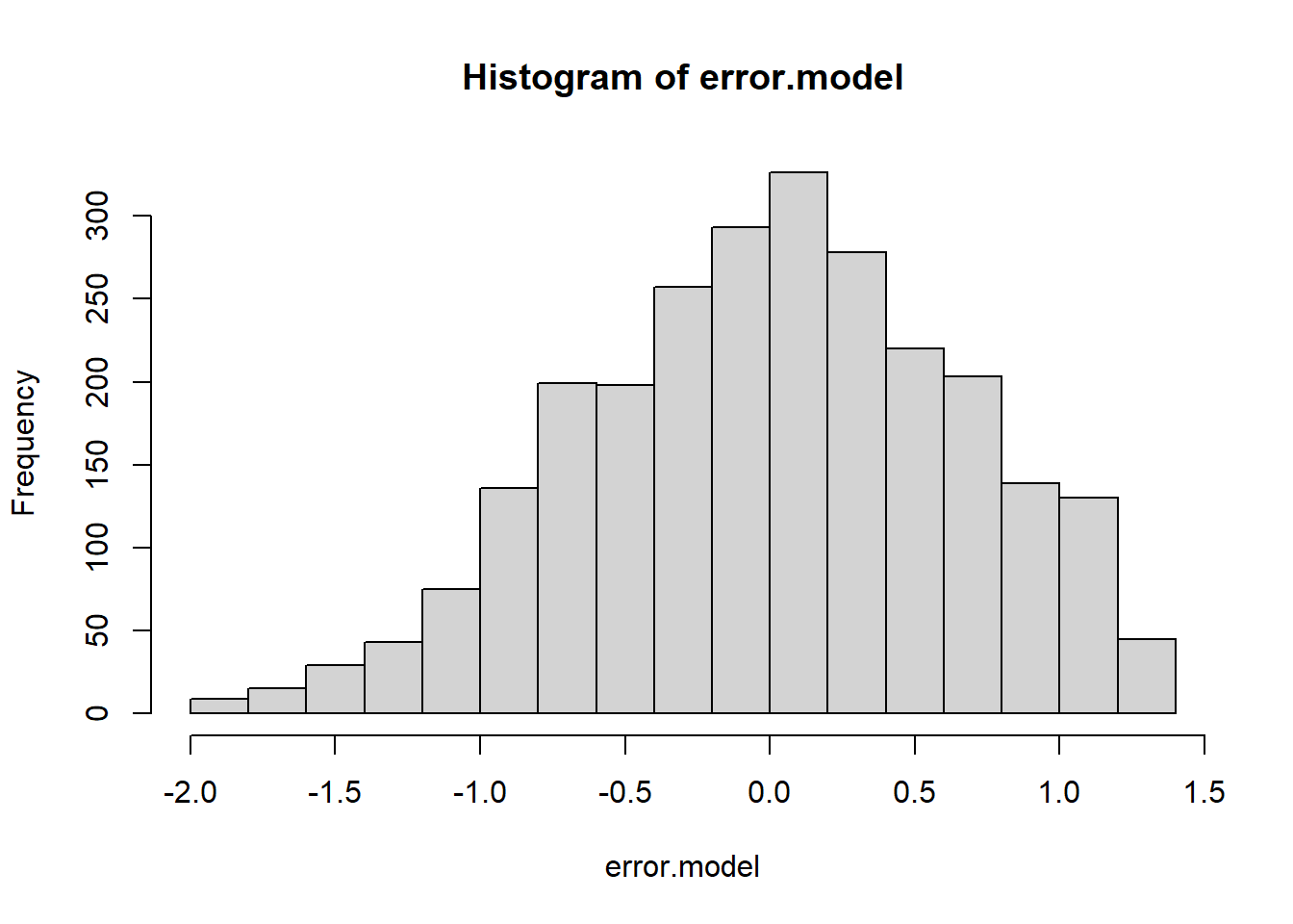
5.3.2.3 Normality of the residuals
As a test for normality, we can (a) look at the distribution of residuals using a histogram, (b) plot a so-called Q-Q plot and interpret it, or (c) look at the distribution of variables in the model using a histogram (note that this can only give an indirect cue about the distribution of errors).
qqPlot(error.model)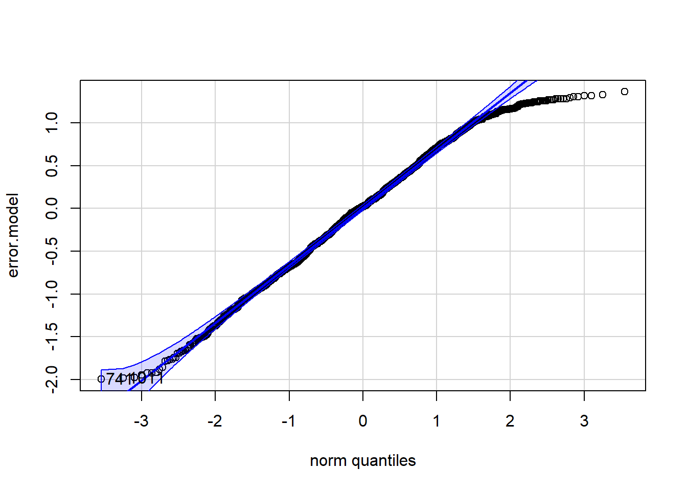
## [1] 741 1011From the visual inspection, the distribution of errors looks similar to a normal distribution. The center of the distribution is about zero and the distribution is only slightly left-skewed.
Regarding the Q-Q plot, the residual values shown should be on (or close to) the line as best as possible. A bit of “fraying” for high or low values is acceptable. We see slight deviations on the right, so there are a little too few values in the positive extreme range. Otherwise, it looks fine.
5.3.2.4 Homoscedasticity
Next, we inspect the assumption of homoscedasticity. We compare the predicted values from the model with the residual values. The more evenly the dots are scattered around the blue line, the more likely we can assume that the assumption is met.
scatterplot(error.model~predict.model, regLine=TRUE, smooth=FALSE, boxplots=FALSE)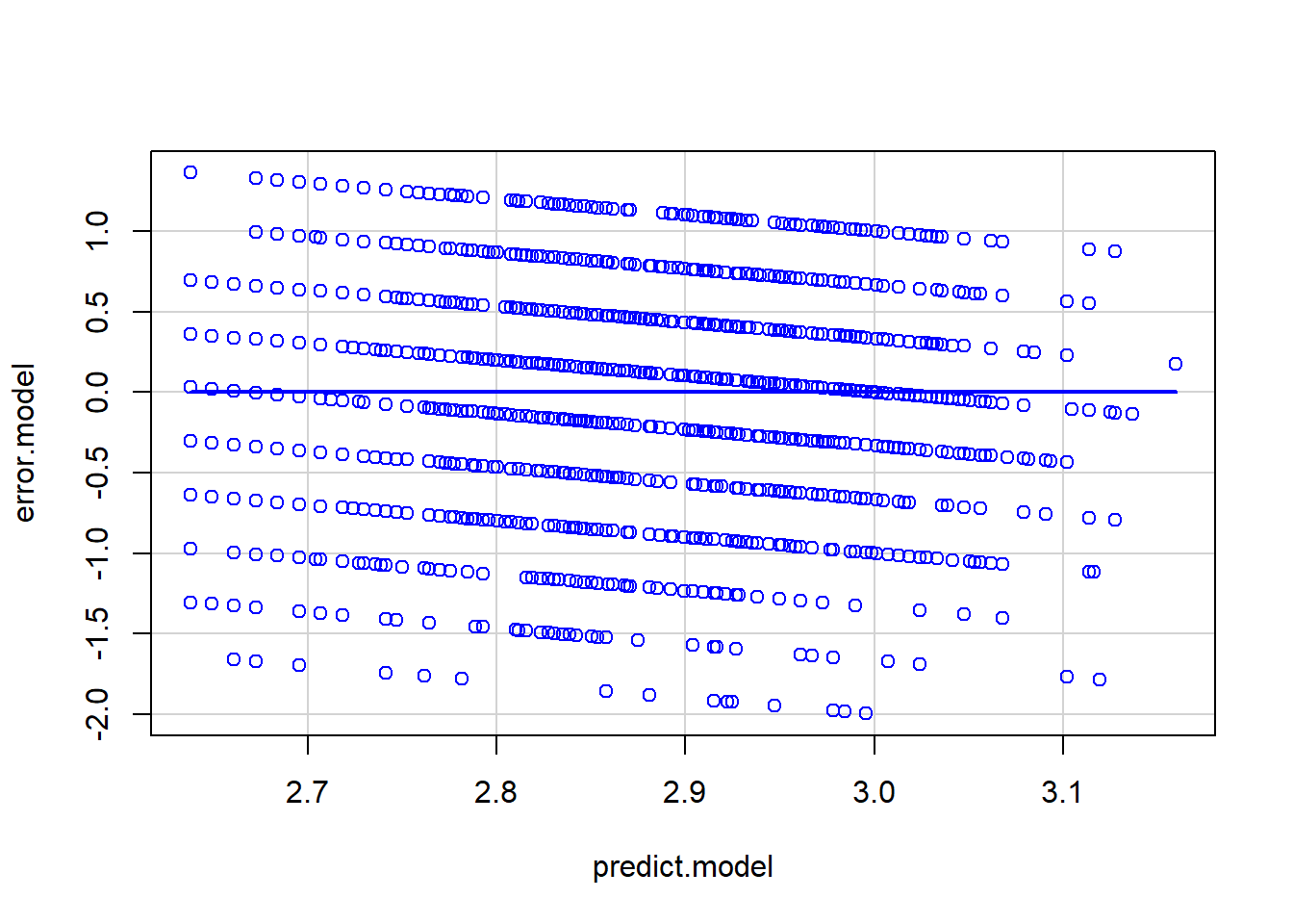
In our case, the errors scatter quite evenly. This means that the model fits similarly at low, medium, and high prediction values. To be certain, we could plot the (standardized) residuals for all independent variables in the model and their ranges of values. Furthermore, there is a statistical test for homoscedasticity: the Breusch-Pagan test. The null hypothesis here would be that homoscedasticity exists (i.e., the residuals are independent of the predictors). A non-significant result is therefore the desired result of the test.
bptest(model_mult)##
## studentized Breusch-Pagan test
##
## data: model_mult
## BP = 5.4228, df = 4, p-value = 0.2466The non-significant result indicates that the assumption of homoscedasticity appears to be met. If this was not the case, we would have to work with robust standard errors.
5.3.3 Non-linear effects
Including a non-linear variable relationship in a regression model can be based on several motives. One reason may be that we may notice from a scatter plot that the relationship between two variables is u-shaped or inversely u-shaped. Another reason might be that we can theoretically reason that the relationship is non-linear. A third motivation is to include non-linear relationships to reduce heteroskedasticity.
Below, we test whether or not income has a non-linear effect on attitudes toward justice. Specifically, we assume that particularly middle-class individuals prefer justice and poor and rich individuals do so less. For rich people, the reason could be self-interest, while people with a low income might oppose redistributive policies because they are afraid of welfare state overuse by newcomers such as immigrants. The latter phenomenon has been discussed in the literature as “welfare chauvinism.”
Let us first look at the relationship graphically.
#Create and print scatter plot
sc1 <- ggplot(data=data_allbus, aes(income, morejustice)) +
  geom_point()
sc1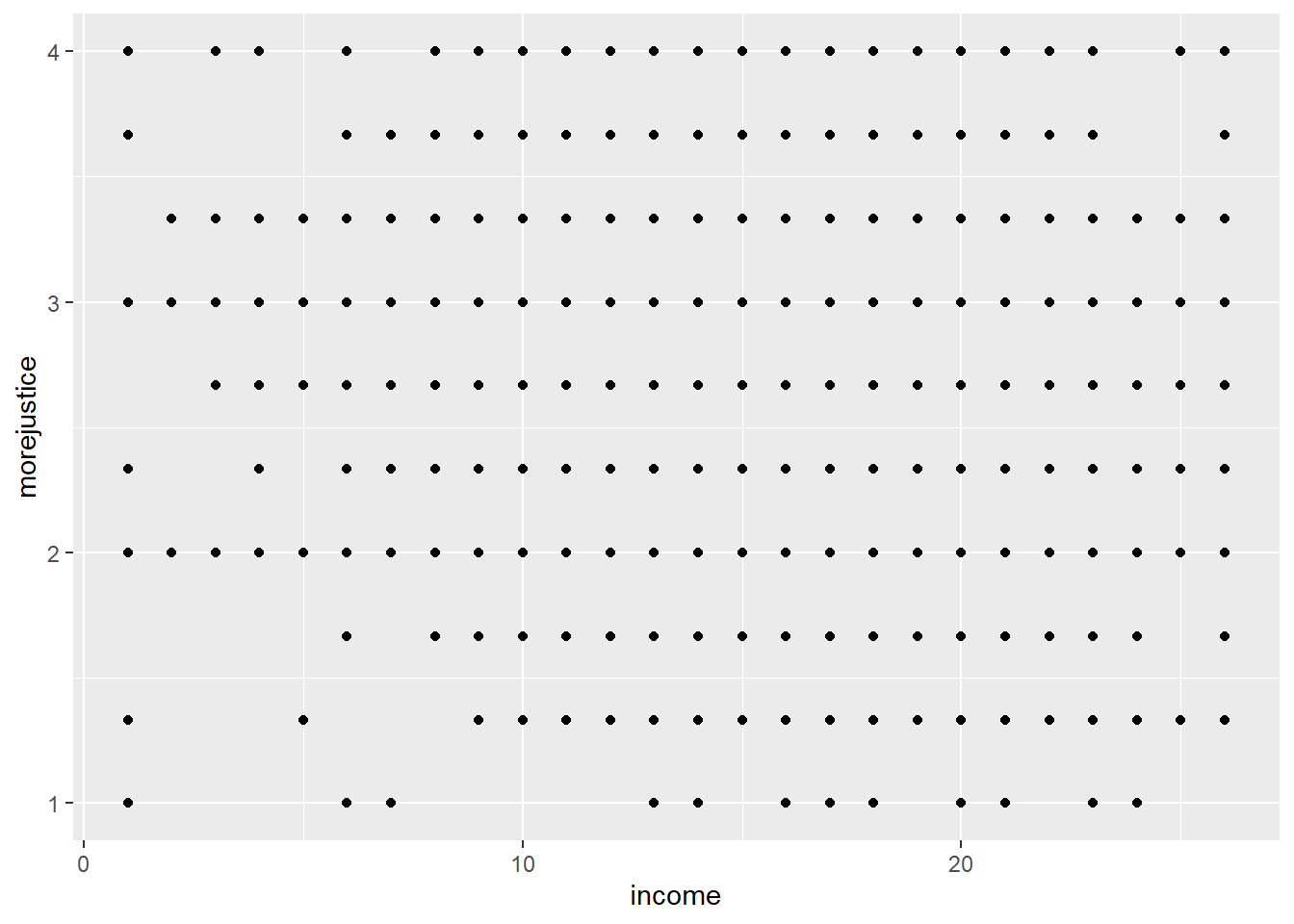
sc2 <- ggplot(data=data_allbus, aes(income, morejustice)) +
  geom_jitter(aes(income = morejustice), size = 0.5) + geom_smooth()
sc2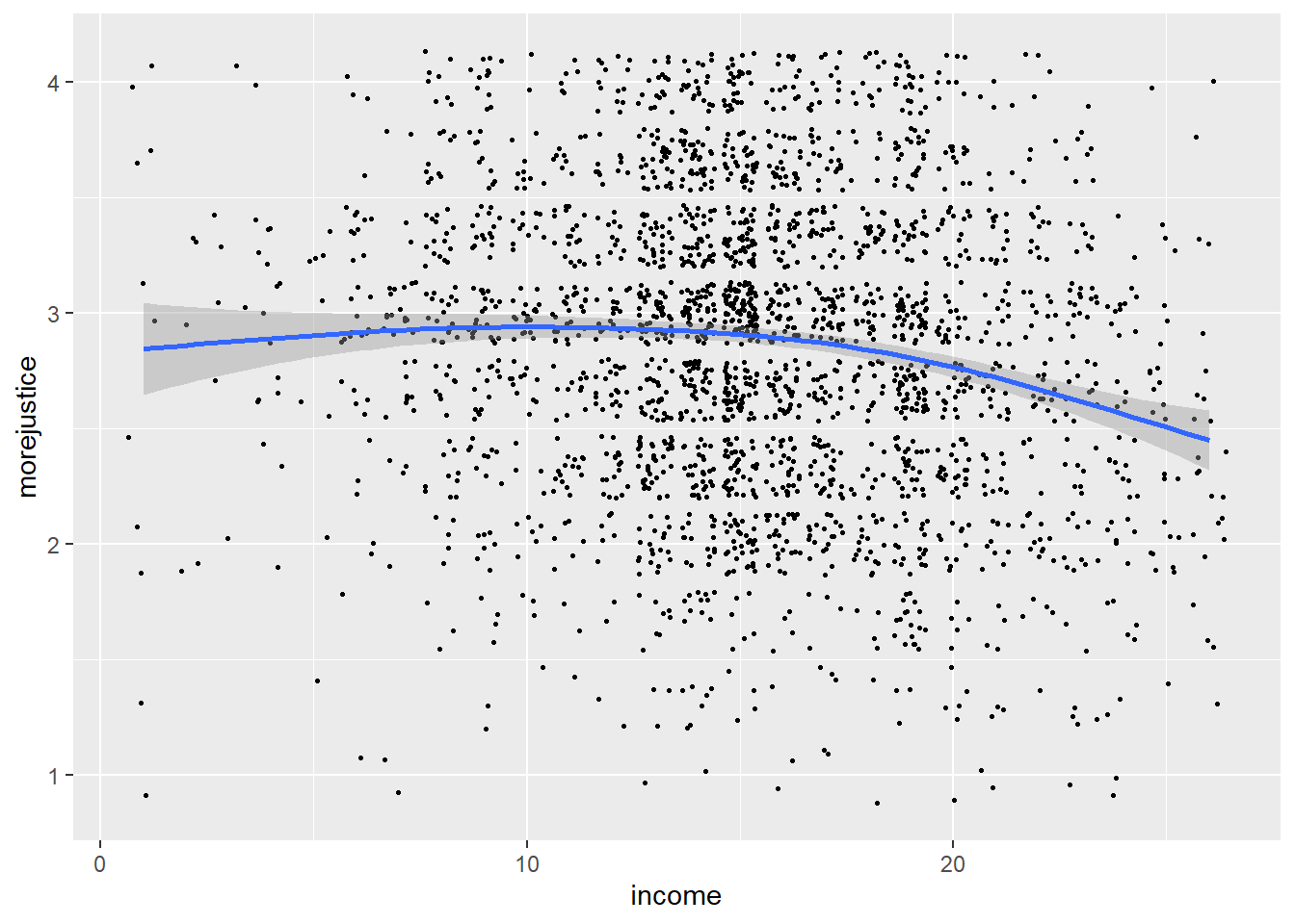
In the first figure, one cannot see a pattern because many points are simply stacked on top of each other. To make the density of the points more visible, we can add a small random fluctuation. This makes the plot somewhat less accurate, but we can now see the pattern, which is also illustrated by the smoothed correlation function (and confidence intervals) represented by the blue line. There is some visual evidence for a non-linear relationship.
We now test for the non-linear relationship in the regression model. To do so, we add the squared variable for income as an additional predictor in the multiple model. The idea here is that the effect of income now depends on the value of “another” variable, namely income itself. In other words, the effect of income on attitudes toward justice is now allowed to vary depending on where you are on the income scale.
data_allbus$income_squared <-  data_allbus$income*data_allbus$income

model_nlin <- lm(morejustice ~ 1 + income + income_squared + female + unemployed + east, data = data_allbus)

stargazer(model_biv, model_mult, model_nlin, type = "text")
##
## ==============================================================================================
## Dependent variable:
## --------------------------------------------------------------------------
## morejustice
## (1) (2) (3)
## ----------------------------------------------------------------------------------------------
## income -0.018*** -0.011*** 0.048***
## (0.003) (0.003) (0.013)
##
## income_squared -0.002***
## (0.0004)
##
## female 0.128*** 0.125***
## (0.028) (0.028)
##
## unemployed 0.066** 0.055*
## (0.033) (0.033)
##
## east 0.075*** 0.058**
## (0.028) (0.028)
##
## Constant 3.141*** 2.936*** 2.546***
## (0.045) (0.059) (0.101)
##
## ----------------------------------------------------------------------------------------------
## Observations 2,595 2,595 2,595
## R2 0.016 0.027 0.036
## Adjusted R2 0.016 0.026 0.034
## Residual Std. Error 0.657 (df = 2593) 0.654 (df = 2590) 0.651 (df = 2589)
## F Statistic 42.484*** (df = 1; 2593) 18.263*** (df = 4; 2590) 19.189*** (df = 5; 2589)
## ==============================================================================================
## Note: *p<0.1; **p<0.05; ***p<0.01Interpretation:
First, we look if the coefficient for the squared variable
income_squaredis statistically significant -> yes, so we can infer a non-linear relationshipNext, we look at the sign of the coefficient of
income-> positiveAnd the sign of the coefficient of
income_squared-> negativeTo summarize: The effect of income on justice attitudes is positive and decreases with higher values of income.
Question: How would the effect be interpreted if both signs were negative?
Your answer:
Solution:
The effect of income on attitudes toward inequality would be negative and decrease for high values of income.
5.3.4 Interaction between two different variables
Another important tool in regression analysis is to model interactions between variables. The idea is that the effect of one variable on the outcome variable depends on the value of another variable in the model. Specifically, the question we ask here is whether the effect of gender on attitudes toward justice differs between West and East Germany. The assumption would be that in East Germany the difference between men and women in justice attitudes is less pronounced than in West Germany. On the one hand, this may be because men in East Germany are more supportive of justice (and thus have similarly high levels of support compared to women). On the other hand, it could be (but this is implausible) that women in the East have similarly “low” values as men.
Let us look at this as an interaction in the regression model. For this, it is important to have the two variables female and east in the model, as well as a variable that is the product of both variables (interaction). This variable can be built beforehand or we build it “on the fly” in R by adding a “:” between two existing variables (“*” also works).
# Letting R know that the two nominal variables "female" and "east" are indeed nominal or "factor variables" is important for the graphical representation of the interaction below

data_allbus$female <- factor(data_allbus$female)
data_allbus$east <- factor(data_allbus$east)

# The interactions can be specified with ":" or "*".
model_interaktion <- lm(morejustice ~ 1 + income + unemployed + female + east + female : east , data = data_allbus)

stargazer(model_interaktion, type = "text")
##
## ===============================================
## Dependent variable:
## ---------------------------
## morejustice
## -----------------------------------------------
## income -0.011***
## (0.003)
##
## unemployed 0.065*
## (0.033)
##
## female1 0.163***
## (0.033)
##
## east1 0.128***
## (0.040)
##
## female1:east1 -0.106*
## (0.056)
##
## Constant 2.912***
## (0.060)
##
## -----------------------------------------------
## Observations 2,595
## R2 0.029
## Adjusted R2 0.027
## Residual Std. Error 0.654 (df = 2589)
## F Statistic 15.351*** (df = 5; 2589)
## ===============================================
## Note: *p<0.1; **p<0.05; ***p<0.01Interpretation:
First, we look to see if the coefficient for the interaction variable
female1:east1is statistically significant -> Yes, so we can assume that the effect offemaleonmorejusticedepends on the value ofeast. In other words, the gender difference in justice attitudes differs between the two parts of Germany. (Note: It would also be correct to interpret the interaction effect symmetrically: The effect ofeastonmorejusticedepends on the value offemale. For simplicity, we do not pursue this interpretation here.)Then, we look at the sign and significance of the coefficient of
female-> positive (= positive effect offemaleifeast= 0, i.e., in West Germany).Then, we look at the sign of the coefficient of the interaction term
woman:east-> negative.To summarize: The positive effect of being a woman on justice attitudes (= gender difference) is less strong (“increasingly negative”) at higher values of
east, i.e., in East Germany.
Below, we see a graphical representation of the package interactions (see https://interactions.jacob-long.com/index.html for more examples).
cat_plot(model_interaktion, pred = female, modx = east, geom = "line", point.shape = TRUE,
         vary.lty = TRUE)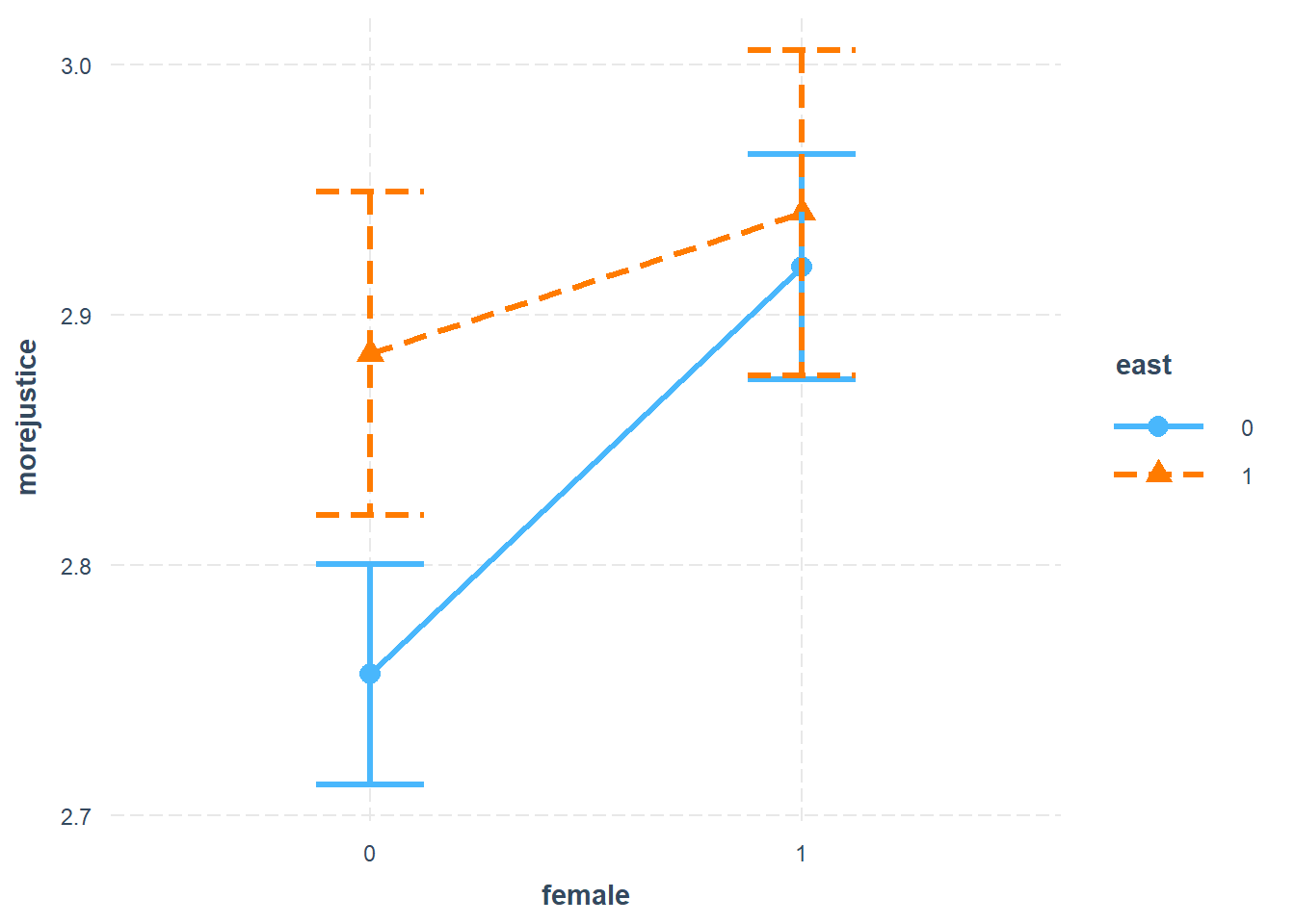
The blue line represents West Germany, and the orange line East Germany. The lines with the bars at the end are 95% confidence intervals, thus indirectly showing how “significant” the respective effects are estimated to be.
Three things stand out:
Women and men in East Germany are more supportive of social justice than women and men in West Germany (orange triangles compared to blue dots). The difference is statistically significant for men in West Germany (confidence intervals on the left side do not overlap). To know whether the overall level of support (women and men combined) is statistically significantly higher in the East, we have to go back to model_mult and look at the average relationship (\(\beta_4 = 0.075, p < 0.01\)).
Looking at the lines and thus the effect of gender separately for both parts of the country, the difference between women and men is statistically significant in West Germany (see coefficient for
female, 0.163). In East Germany, the difference is not significant. (This can also be visually inferred by comparing the orange and the blue estimates to each other.)The effect of being a woman is larger in West Germany than in East Germany (the blue line is steeper than the orange line). This is represented by the coefficient for the interaction term.
We can now insert the regression coefficients into a regression formula:
\(y = \beta_0 + \beta_1 * x_1 + \beta_2 * x_2 + \beta_3 * x_3 + \beta_4 * x_4 + \beta_5 * x_3*x_4 + e\)
\(morejustice = 2.912 - 0.011 * income + 0.065 * unemployed + 0.163*female + 0.128*east - 0.106*female*east + e\)
We can also derive the formulas for the so-called marginal effects by taking the first derivative and entering the variable values in a combination that informs us about the effects for the different groups.
- Marginal Effect for the variable
east(first derivative) \(dy/d(east) = 0.128 – 0.106*female\)
We can substitute 0 for the variable female, i.e., the effect of
eastfor men: \(b(east=1, female=0) = 0.128 – 0.106 * 0 = 0.128\).This refers to the difference between East and West in men (plot: distance between blue dot and orange triangle on the left).
If we substitute 1 for the variable female: i.e., the effect of
eastfor women: \(b(east=1, female=1) = 0.128 – 0.106 * 1 = 0.022\).This refers to the small difference between East and West in women (distance between blue dot and orange triangle on the right side).
- Marginal Effect for the variable
female(first derivative) \(dy/d(female) = 0.163 – 0.106*east\)
We can substitute 0 for the variable east, i.e., the effect of
femalefor West Germans: \(b(female=1, east=0) = 0.163 – 0.106 * 0 = 0.163\).This refers to the difference between women and men in West Germany (plot: distance between both blue dots).
If we substitute 1 for the variable east, i.e., the effect of
femalefor East Germans: \(b(female=1, east=1) = 0.163 – 0.106 * 1 = 0.057\).This refers to the difference between women and men in East Germany (distance between both orange triangles).
- The effect difference of women (different in both slopes) is represented by the coefficient for the interaction, i.e., –0.106.
Thank you for engaging with the Introduction to Statistics and Data Analysis - A Case-Based Approach!
Feedback to conrad.ziller@uni-due.de is much appreciated.