5 Results
5.1 Exploratory Data Analysis
5.1.1 Descriptive Statistics
pheno_qc %>%
  group_by(Subgroup_Number, Subgroup) %>%
  summarise(N = n(),
            Mean = round(mean(Age), 1),
            Median = median(Age),
            SD = round(sd(Age), 2),
            Minimum = min(Age),
            Maximum = max(Age)) %>%
  rename(`Subgroup` = Subgroup_Number,
         `Genetic lines` = Subgroup) %>%
  kable(.,
        row.names = FALSE,
        align = 'c',
caption = "Descriptive statistics AGE by subgroup after genotype quality control.")| Subgroup | Genetic lines | N | Mean | Median | SD | Minimum | Maximum |
|---|---|---|---|---|---|---|---|
| 1 | Crossbred | 8447 | 142.8 | 142 | 17.20 | 110 | 164 |
| 2 | Duroc | 16633 | 144.9 | 144 | 20.47 | 55 | 171 |
| 3 | Landrace | 18834 | 143.2 | 145 | 19.50 | 55 | 171 |
| 4 | Yorkshire | 17764 | 143.3 | 145 | 19.36 | 60 | 171 |
| 5 | Crossbred and Duroc | 25091 | 144.2 | 144 | 19.46 | 55 | 171 |
| 6 | Crossbred and Landrace | 27281 | 143.1 | 144 | 18.82 | 55 | 171 |
| 7 | Crossbred and Yorkshire | 26221 | 143.1 | 144 | 18.70 | 60 | 171 |
| 8 | Duroc and Landrace | 35480 | 144.0 | 145 | 19.98 | 55 | 171 |
| 9 | Duroc and Yorkshire | 34417 | 144.0 | 144 | 19.93 | 55 | 171 |
| 10 | Landrace and Yorkshire | 36609 | 143.2 | 145 | 19.43 | 55 | 171 |
| 11 | Duroc, Landrace, and Yorkshire | 53256 | 143.7 | 145 | 19.78 | 55 | 171 |
| 12 | Crossbred, Duroc, Landrace, and Yorkshire | 61702 | 143.6 | 144 | 19.45 | 55 | 171 |
5.1.2 Raw Distributions
5.1.2.1 One Breed
ggplot(filter(pheno_qc, Subgroup_Code %in% c("c", "d", "l", "y")), aes(x=Age)) +
  geom_histogram(color="white", fill="steelblue1", position = "dodge") +
  facet_wrap(~Subgroup, nrow = 2) +
  scale_x_continuous(expand = c(0,3)) +
  scale_y_continuous(expand = c(0,0), limits = c(0, 4000)) +
  geom_hline(yintercept = 0) +
  labs(y = "No. of pigs", x = "Age, months") +
  theme_classic() +
  theme(strip.background = element_rect(fill="grey70")) +
  theme(strip.text = element_text(color = 'white', face = "bold", size = "12"),
        axis.title = element_text(face = "bold"))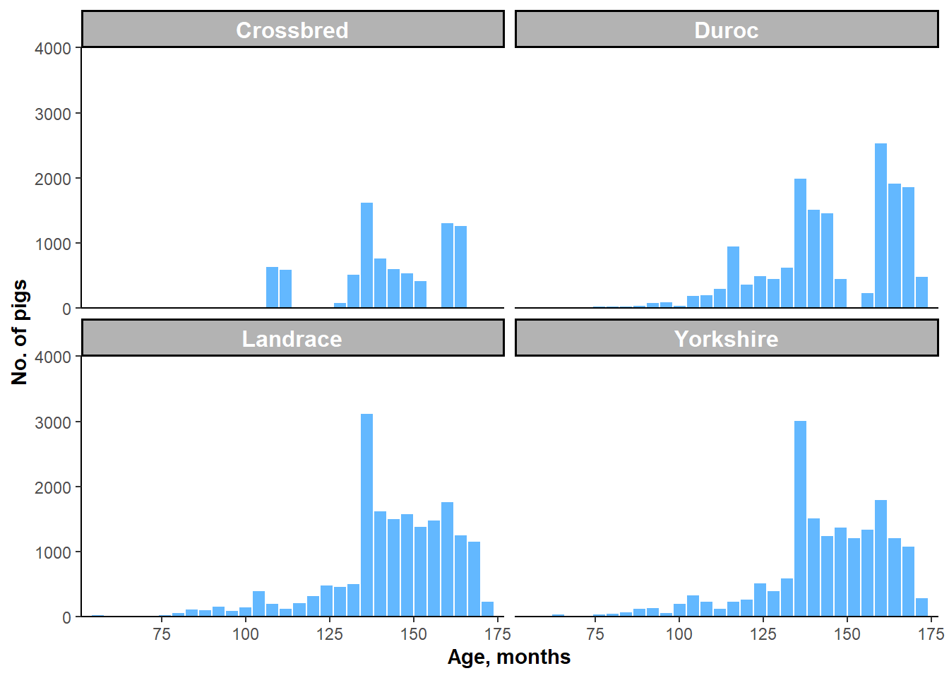
Figure 5.1: Histograms of AGE by one-breed subgroups.
5.1.2.2 Two Breeds
ggplot(filter(pheno_qc, Subgroup_Code %in% c("cd", "cl", "cy", "dl", "dy", "ly")), aes(x=Age)) +
  geom_histogram(color="white", fill="steelblue1", position = "dodge") +
  facet_wrap(~Subgroup, nrow = 3) +
  scale_x_continuous(expand = c(0,3)) +
  scale_y_continuous(expand = c(0,0), limits = c(0, 4000)) +
  geom_hline(yintercept = 0) +
  labs(y = "No. of pigs", x = "Age, months") +
  theme_classic() +
  theme(strip.background = element_rect(fill="grey70")) +
  theme(strip.text = element_text(color = 'white', face = "bold", size = "12"),
        axis.title = element_text(face = "bold"))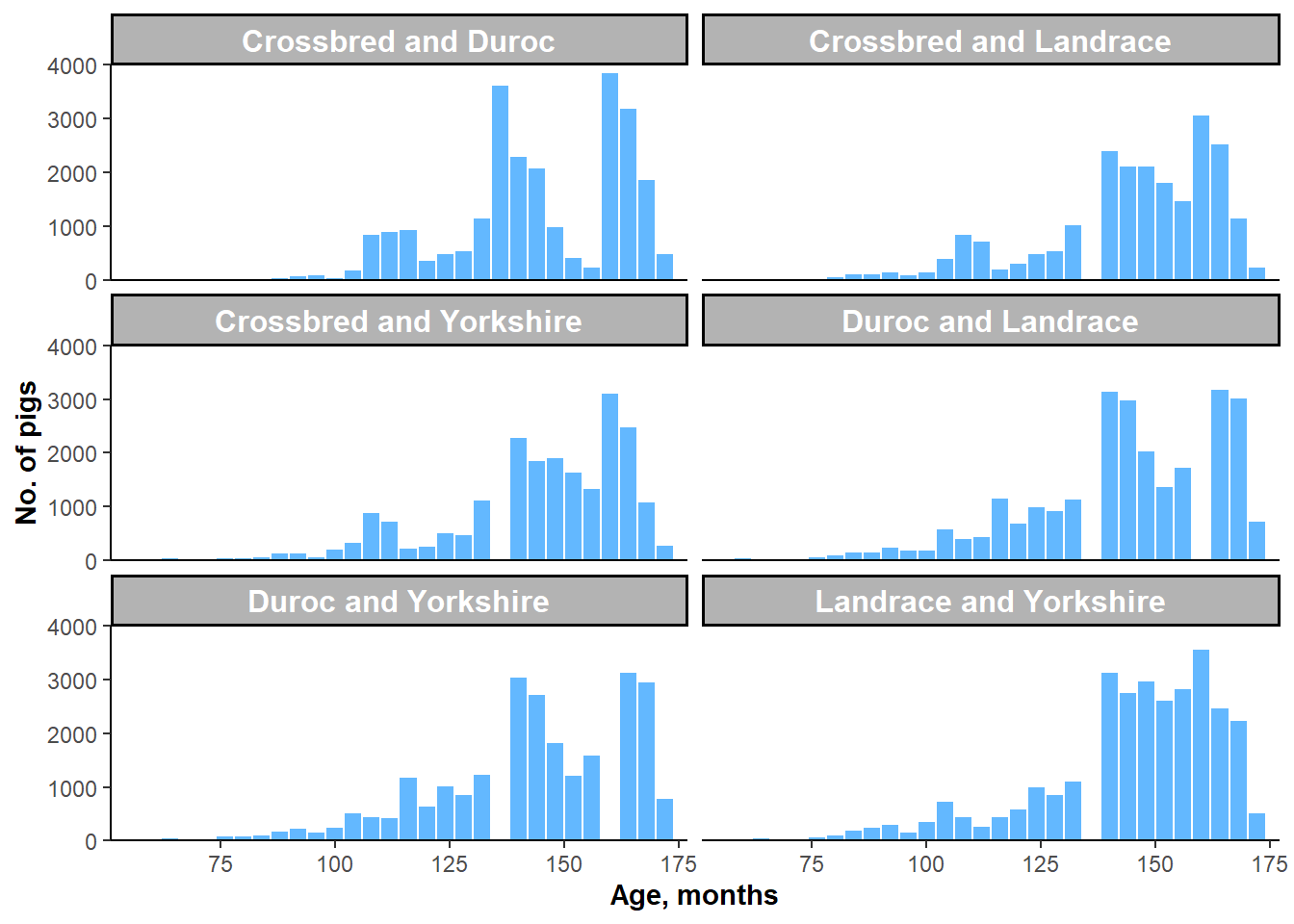
Figure 5.2: Histograms of AGE by two-breed subgroups.
5.1.2.3 Three+ Breeds
ggplot(filter(pheno_qc, Subgroup_Code %in% c("dly", "cdly")), aes(x=Age)) +
  geom_histogram(color="white", fill="steelblue1", position = "dodge") +
  facet_wrap(~Plot_Code, nrow = 1) +
  scale_x_continuous(expand = c(0,3)) +
  scale_y_continuous(expand = c(0,0), limits = c(0, 5000)) +
  geom_hline(yintercept = 0) +
  labs(y = "No. of pigs", x = "Age, months") +
  theme_classic() +
  theme(strip.background = element_rect(fill="grey70")) +
  theme(strip.text = element_text(color = 'white', face = "bold", size = "12"),
        axis.title = element_text(face = "bold"))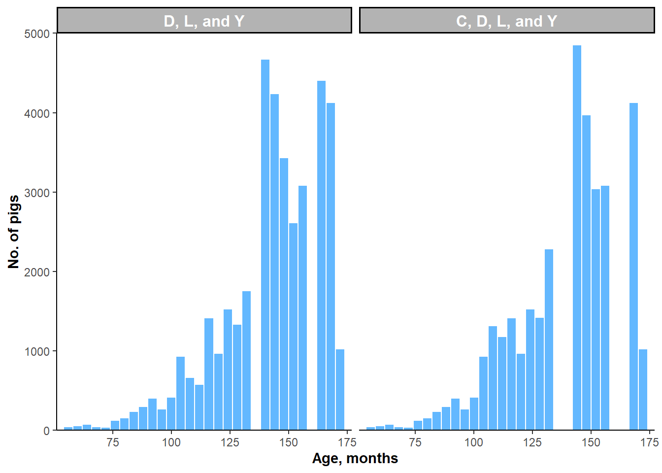
Figure 5.3: Histograms of AGE by subgroups of three or more breeds.
5.2 Univariate Variance Component Estimation
uvce <- read.csv("results/uvce.csv",
                 header = TRUE)
uvce$Breeds_N <- factor(uvce$Breeds_N,
                        levels = c("One Breed", "Two Breeds", "Three+ Breeds"))
uvce$Plot_Code <- factor(uvce$Plot_Code,
                             levels = c("C", "D", "L", "Y", "C and D", "C and L", "C and Y", "D and L", "D and Y", "L and Y", "D, L, and Y", "C, D, L, and Y"))

library(RColorBrewer)
ggplot(uvce, aes(x = Plot_Code, y = PVE, color = SNP_Group)) +
  geom_point(aes(size = Pigs_n)) +
  scale_y_continuous(limits = c(0,1), breaks = round(seq(0, 1, by = 0.1), 2), expand = c(0,0)) +
  labs(x = "Subgroup", y = "Proportion of Variance Explained by SNPs",
       color = "GRM", size = "Sample Size") +
  theme_light() +
  theme(axis.text.x = element_text(angle = 45, vjust = .5),
        axis.title = element_text(face = "bold"),
        strip.background = element_rect(fill="grey70"),
        strip.text = element_text(color = 'white', face = "bold", size = "12"),
        legend.title = element_text(face = "bold")) +
  facet_grid(~Breeds_N, scales = "free") +
  scale_color_brewer(palette="RdBu")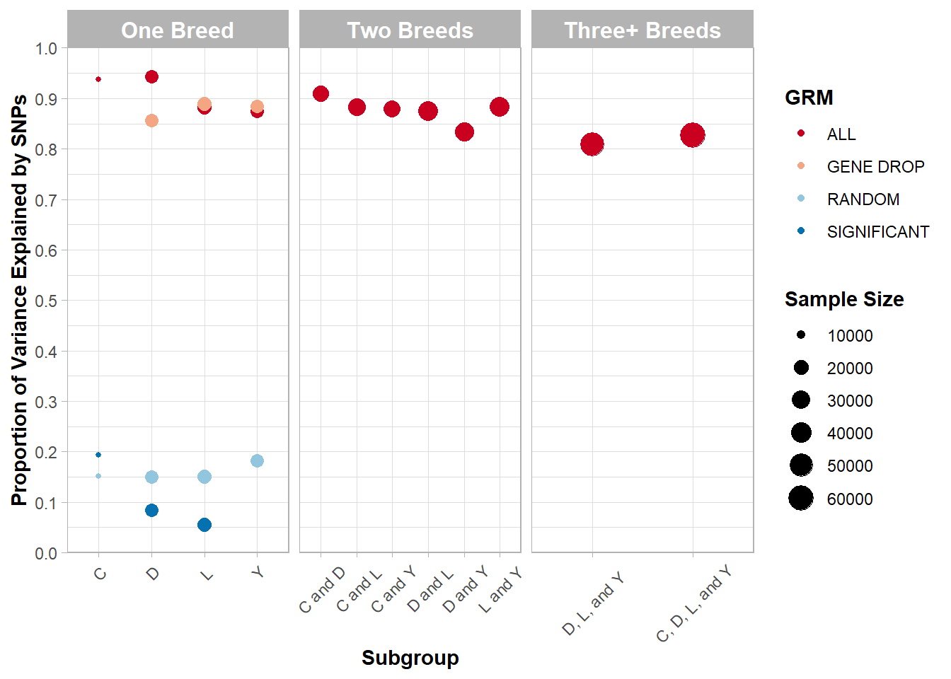
Figure 5.4: Proportion of variance in AGE explained by SNPs across various subgroups and subsets of SNPs.
5.3 Bivariate Variance Component Estimation
bvce <- read.csv("results/bvce.csv",
                 header = TRUE)
bvce$Plot_Code <- factor(bvce$Plot_Code,
                             levels = c("C", "D", "L", "Y", "C and D", "C and L", "C and Y", "D and L", "D and Y", "L and Y", "D, L, and Y", "C, D, L, and Y"))

ggplot(bvce, aes(x = Plot_Code, y = rG, color = SNP_Group, shape = Breed)) +
  geom_point(size = 4) +
  scale_y_continuous(limits = c(-0.2,1), breaks = round(seq(-0.2, 1, by = 0.1), 2), expand = c(0,0)) +
  labs(x = "Subgroup", y = "Genetic correlation (rG)",
       color = "SNP Group", shape = "GRM") +
  theme_light() +
  theme(axis.text.x = element_text(angle = 45, vjust = .5),
        axis.title = element_text(face = "bold"),
        strip.background = element_rect(fill="grey70"),
        strip.text = element_text(color = 'white', face = "bold", size = "12"),
        legend.title = element_text(face = "bold")) +
  scale_color_brewer(palette="RdBu") +
  geom_hline(yintercept = 0, size = 1)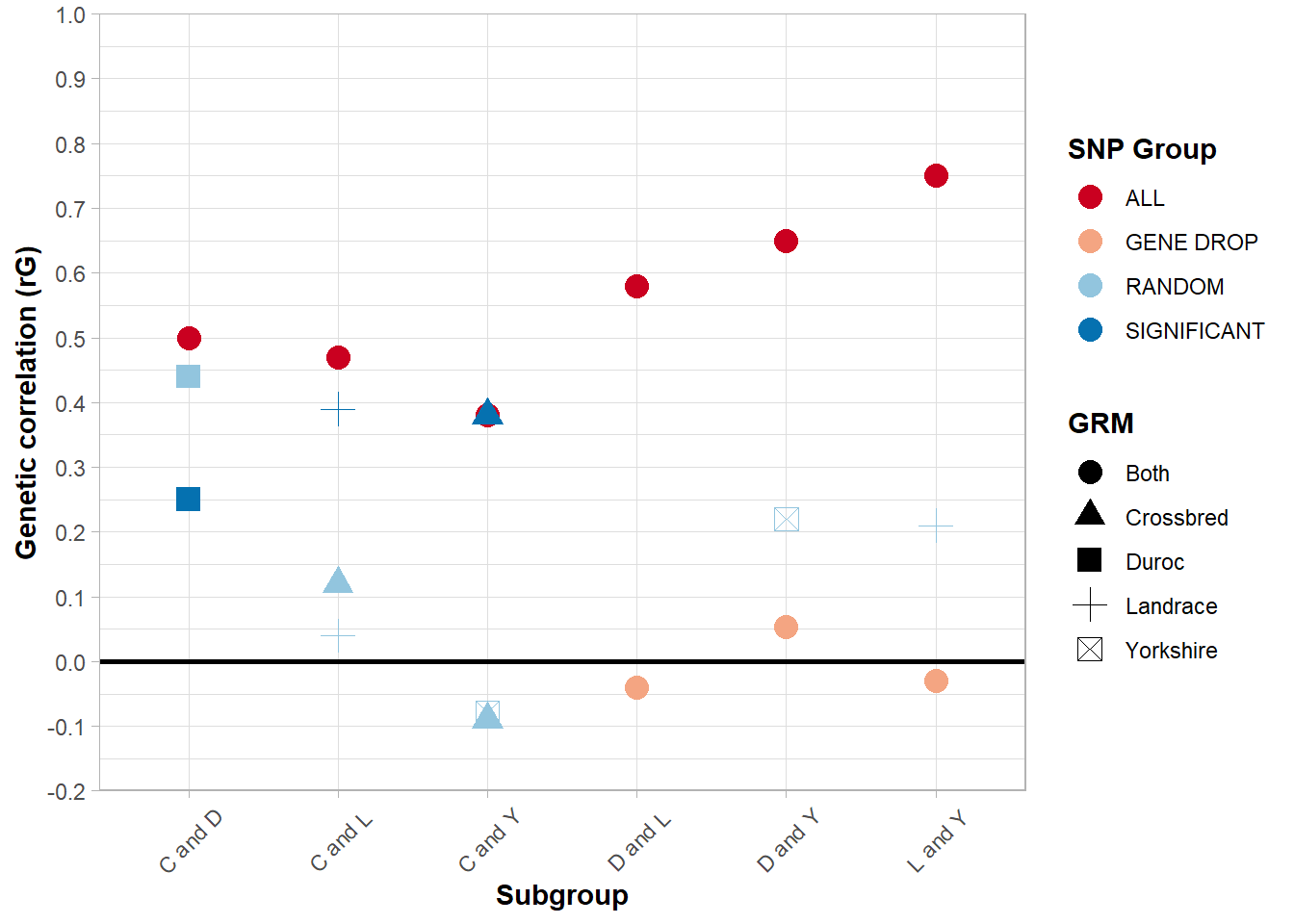
Figure 5.5: Genetic correlation between breeds for AGE across various subgroups and subsets of SNPs.
5.4 Genome-wide Association Analyses
5.4.1 Frequency of Detected Associations
mlma %>%
  mutate(Threshold = 0.05,
         Adjusted_Threshold = Threshold/SNPs_n,
         p_sig = p < Adjusted_Threshold,
         q_sig = q < 0.10) %>%
  group_by(Subgroup_Number, Subgroup, Pigs_n, SNPs_n) %>%
  summarise(N_p = sum(p_sig),
            N_q = sum(q_sig)) %>%
  rename(`Subgroup` = Subgroup_Number,
         `Genetic lines` = Subgroup,
         `Pigs, n` = Pigs_n,
         `SNPs, n` = SNPs_n,
         `Signifigant SNPs (Bonferroni), n` = N_p,
         `Signifigant SNPs (Q-value), n` = N_q) %>%
  kable(.,
        row.names = FALSE,
        align = 'c',
caption = "Number of statistically significant SNPs per subgroup based on Bonferroni (alpha/N, SNPs) and Q-value (Q < 0.10) thresholds.")| Subgroup | Genetic lines | Pigs, n | SNPs, n | Signifigant SNPs (Bonferroni), n | Signifigant SNPs (Q-value), n |
|---|---|---|---|---|---|
| 1 | Crossbred | 8447 | 46529 | 23 | 49 |
| 2 | Duroc | 16633 | 38377 | 41 | 98 |
| 2 | Simulated Duroc | 16633 | 38376 | 0 | 0 |
| 3 | Landrace | 18834 | 45316 | 56 | 134 |
| 3 | Simulated Landrace | 18834 | 45324 | 0 | 0 |
| 4 | Simulated Yorkshire | 17764 | 45198 | 0 | 0 |
| 4 | Yorkshire | 17764 | 45196 | 51 | 121 |
| 5 | Crossbred and Duroc | 25091 | 46348 | 77 | 147 |
| 6 | Crossbred and Landrace | 27281 | 46431 | 72 | 178 |
| 7 | Crossbred and Yorkshire | 26221 | 46426 | 72 | 169 |
| 8 | Duroc and Landrace | 35480 | 46064 | 177 | 486 |
| 9 | Duroc and Yorkshire | 34417 | 46143 | 215 | 554 |
| 10 | Landrace and Yorkshire | 36609 | 46236 | 76 | 250 |
| 11 | Duroc, Landrace, and Yorkshire | 53256 | 46421 | 250 | 865 |
| 12 | Crossbred, Duroc, Landrace, and Yorkshire | 61702 | 46453 | 297 | 1202 |
5.4.2 Allele Substitution Effects
top_betas <- mlma %>%
  filter(Subgroup_Code %in% c("c", "d", "l", "y")) %>%
  filter(q < 0.10) %>%
  group_by(Plot_Code) %>%
  slice_max(order_by = b, n = 10) %>%
  arrange(-b)

top_betas %>%
  mutate(SNP = reorder(SNP, b)) %>%
  group_by(Subgroup, SNP) %>%
  arrange(b) %>%
  ungroup() %>%
  mutate(SNP = factor(paste(SNP, Subgroup, sep = "__"),
                       levels = rev(paste(SNP, Subgroup, sep = "__")))) %>%
ggplot(., aes(x = SNP, y = b)) +
  geom_errorbar(aes(ymin = b - se*1.96, ymax = b + se*1.96), color = "black", width = .5) +
  geom_point(aes(color = Subgroup), size = 2) +
  facet_wrap(~Subgroup, scales = "free_x") +
  scale_x_discrete(labels = function(x) gsub("__.+$", "", x)) +
  scale_y_continuous(limits = c(0,15)) +
  scale_color_brewer(palette = "RdBu") +
  theme_light() +
  theme(axis.text.x = element_text(angle = 45, vjust = .5),
        axis.title = element_text(face = "bold"),
        strip.background = element_rect(fill="grey70"),
        strip.text = element_text(color = 'white', face = "bold", size = "12"),
        legend.position = "none")  +
  geom_hline(yintercept = 0, size = 1) +
  labs(y = "Allele Substitution Effect (beta)")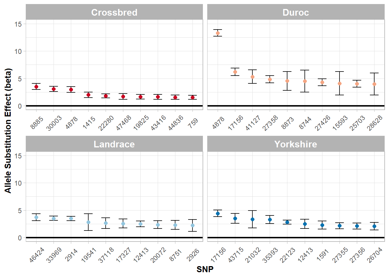
Figure 5.6: Top allele substitution effects (beta) by one breed subgroups.
top_betas <- mlma %>%
  filter(Subgroup_Code %in% c("cd", "cl", "cy", "dl", "dy", "ly")) %>%
  filter(q < 0.10) %>%
  group_by(Plot_Code) %>%
  slice_max(order_by = b, n = 10) %>%
  arrange(-b)

top_betas %>%
  mutate(SNP = reorder(SNP, b)) %>%
  group_by(Plot_Code, SNP) %>%
  arrange(b) %>%
  ungroup() %>%
  mutate(SNP = factor(paste(SNP, Plot_Code, sep = "__"),
                       levels = rev(paste(SNP, Plot_Code, sep = "__")))) %>%
ggplot(., aes(x = SNP, y = b)) +
  geom_errorbar(aes(ymin = b - se*1.96, ymax = b + se*1.96), color = "black", width = .5) +
  geom_point(aes(color = Plot_Code), size = 2) +
  facet_wrap(~Plot_Code, scales = "free_x") +
  scale_x_discrete(labels = function(x) gsub("__.+$", "", x)) +
  scale_y_continuous(limits = c(0,13)) +
  scale_color_brewer(palette = "RdBu") +
  theme_light() +
  theme(axis.text.x = element_text(angle = 45, vjust = .5),
        axis.title = element_text(face = "bold"),
        strip.background = element_rect(fill="grey70"),
        strip.text = element_text(color = 'white', face = "bold", size = "12"),
        legend.position = "none")  +
  geom_hline(yintercept = 0, size = 1) +
  labs(y = "Allele Substitution Effect (beta)")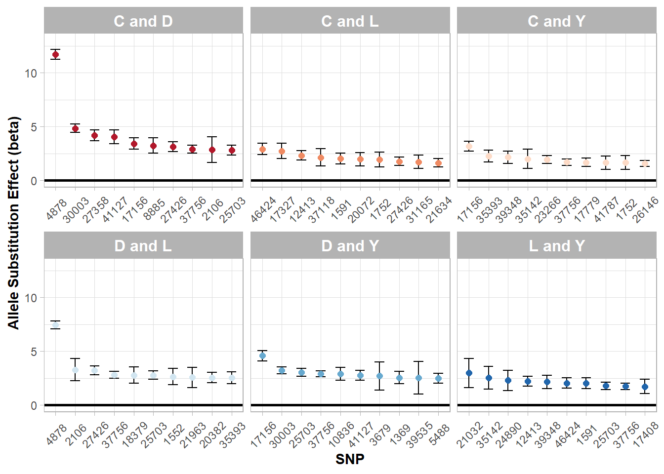
Figure 5.7: Top allele substitution effects (beta) by two breed subgroups.
top_betas <- mlma %>%
  filter(Subgroup_Code %in% c("dly", "cdly")) %>%
  filter(q < 0.10) %>%
  group_by(Plot_Code) %>%
  slice_max(order_by = b, n = 10) %>%
  arrange(-b)

top_betas$Plot_Code <- factor(top_betas$Plot_Code,
                              levels = c("D, L, and Y", "C, D, L, and Y"))

top_betas %>%
  mutate(SNP = reorder(SNP, b)) %>%
  group_by(Plot_Code, SNP) %>%
  arrange(b) %>%
  ungroup() %>%
  mutate(SNP = factor(paste(SNP, Plot_Code, sep = "__"),
                       levels = rev(paste(SNP, Plot_Code, sep = "__")))) %>%
ggplot(., aes(x = SNP, y = b)) +
  geom_errorbar(aes(ymin = b - se*1.96, ymax = b + se*1.96), color = "black", width = .5, size = .7) +
  geom_point(aes(color = Plot_Code), size = 2.5) +
  facet_wrap(~Plot_Code, scales = "free_x") +
  scale_x_discrete(labels = function(x) gsub("__.+$", "", x)) +
  scale_y_continuous(limits = c(0,5)) +
  scale_color_manual(values = c("firebrick3", "royalblue4")) +
  theme_light() +
  theme(axis.text.x = element_text(angle = 45, vjust = .5),
        axis.title = element_text(face = "bold"),
        strip.background = element_rect(fill="grey70"),
        strip.text = element_text(color = 'white', face = "bold", size = "12"),
        legend.position = "none")  +
  geom_hline(yintercept = 0, size = 1) +
  labs(y = "Allele Substitution Effect (beta)")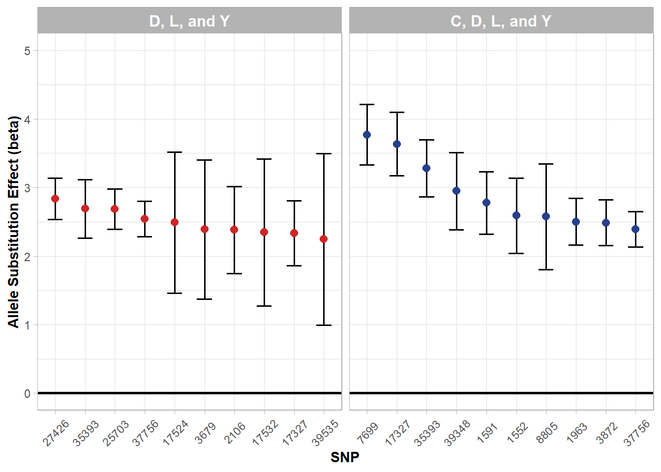
Figure 5.8: Top allele substitution effects (beta) by three+ breed subgroups.
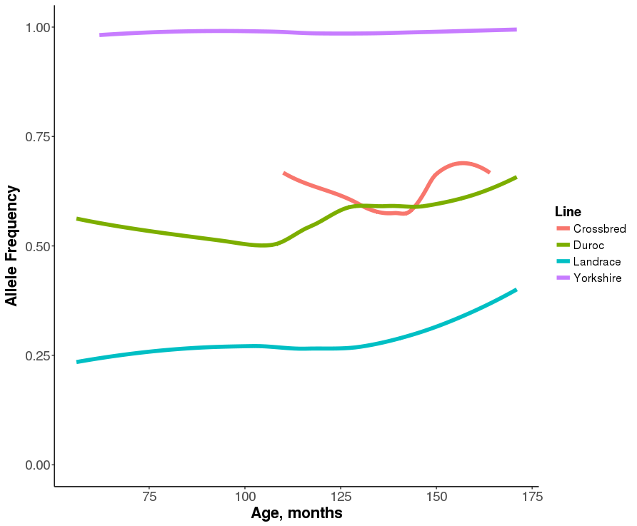
Figure 5.9: Allele frequency changes over time for alleles with the largest allele substitution effect within each one breed subgroup.
5.5 QTL Enrichment
load("QTL_Enrich_Results.RData")
QTLenrich_plot(filter(qtl.enrich, Line == "All") %>%
                 top_n(15, -adj.pval), x = "QTL", pval = "adj.pval")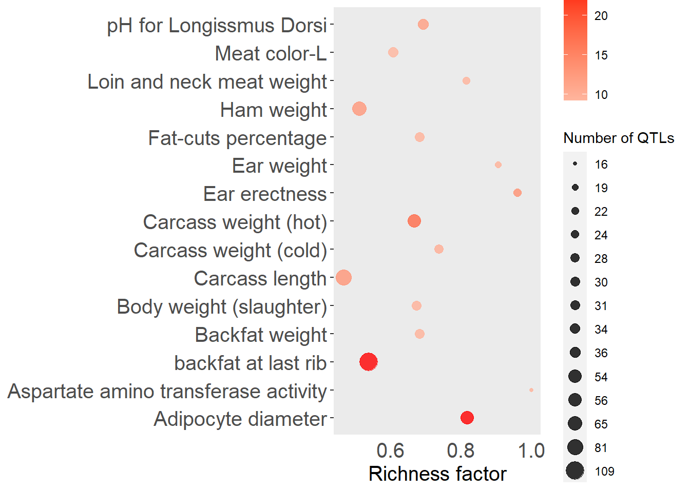
Figure 5.10: Top 15 QTLs by enrichment P-value for the entire group of genotyped pigs.
load("QTL_Enrich_Results.RData")
QTLenrich_plot(filter(qtl.enrich, Line == "1006") %>%
                 top_n(15, -adj.pval), x = "QTL", pval = "adj.pval")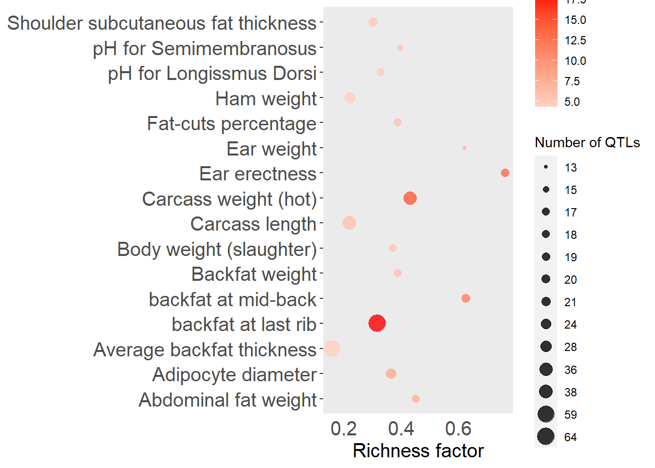
Figure 5.11: Top 15 QTLs by enrichment P-value for the Duroc subgroup.
load("QTL_Enrich_Results.RData")
QTLenrich_plot(filter(qtl.enrich, Line == "10") %>%
                 top_n(15, -adj.pval), x = "QTL", pval = "adj.pval")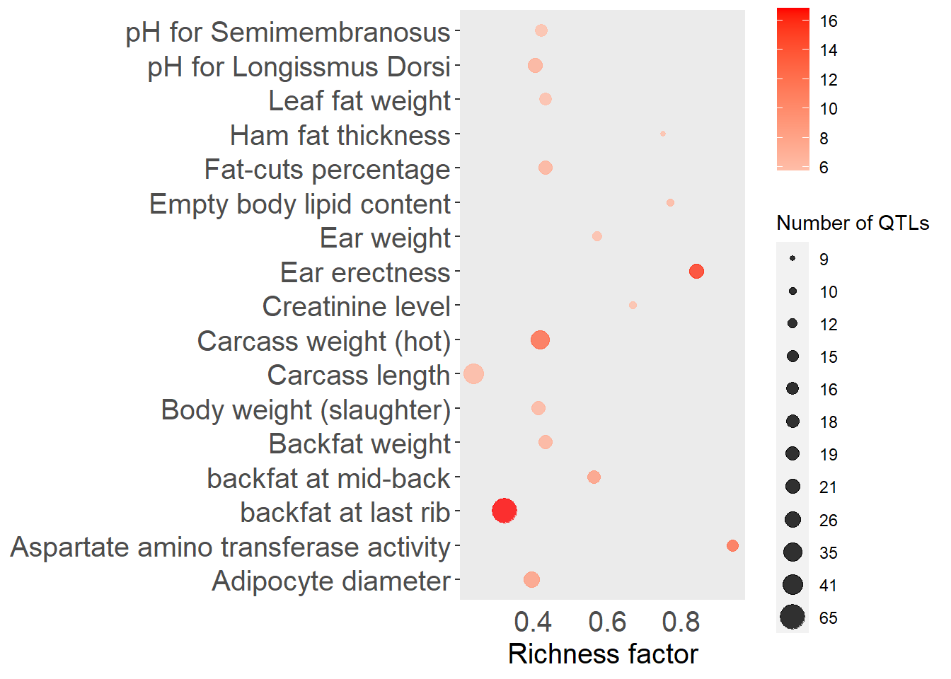
Figure 5.12: Top 15 QTLs by enrichment P-value for the Landrace subgroup.
load("QTL_Enrich_Results.RData")
QTLenrich_plot(filter(qtl.enrich, Line == "11") %>%
                 top_n(15, -adj.pval), x = "QTL", pval = "adj.pval")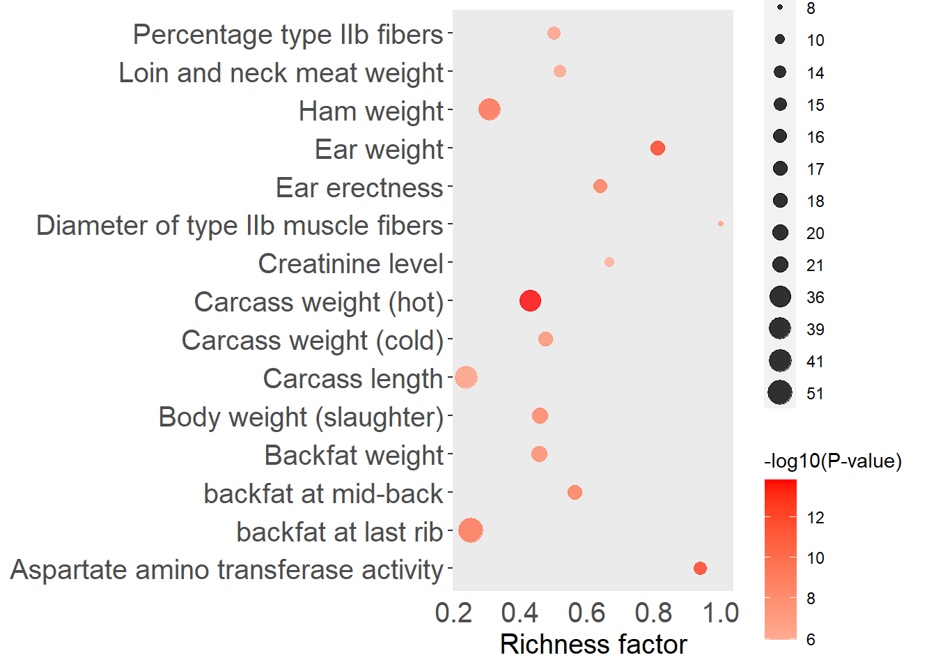
Figure 5.13: Top 15 QTLs by enrichment P-value for the Yorkshire subgroup.
5.6 Gene Enrichment
load("GeneAnnotation.RData")

gene_list <- gene.annotation %>%
  filter(Breed == "All") %>%
  select(gene_id)
gene_list <- gene_list$gene_id

gostres <- gost(query = gene_list,
                organism = "sscrofa", ordered_query = FALSE,
                multi_query = FALSE, significant = TRUE, exclude_iea = FALSE,
                measure_underrepresentation = FALSE, evcodes = FALSE,
                user_threshold = 0.05, correction_method = "fdr",
                domain_scope = "annotated", custom_bg = NULL,
                numeric_ns = "", sources = NULL, as_short_link = FALSE)

gostplot(gostres, capped = FALSE, interactive = FALSE)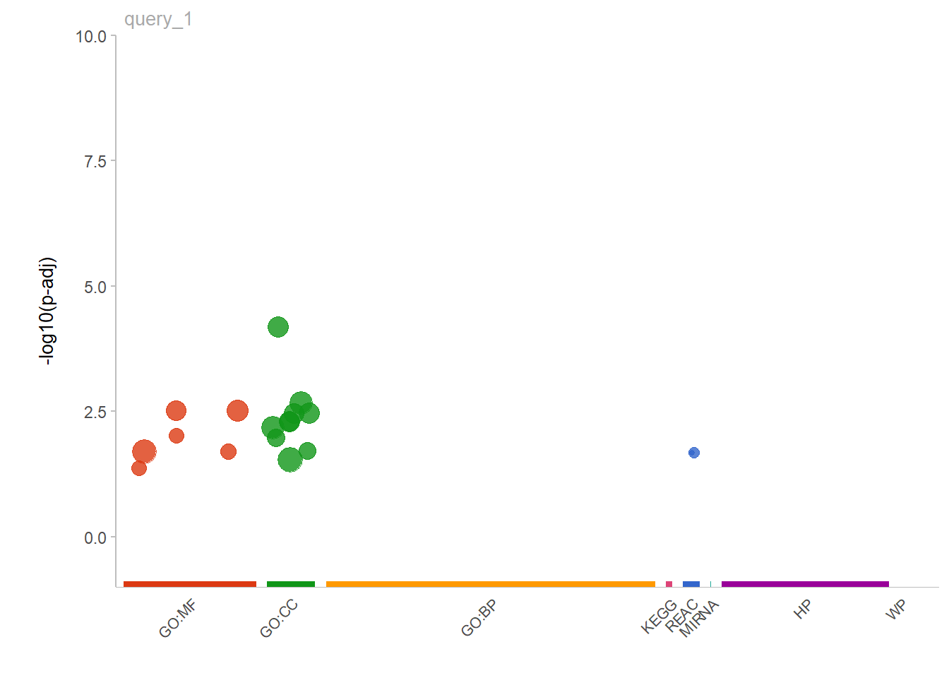
Figure 5.14: Gene Ontology enrichment chart for the entire group of genotyped pigs.
publish_gosttable(gostres, highlight_terms = gostres$result,
                        use_colors = TRUE,
                        show_columns = c("source", "term_name", "term_size", "intersection_size"),
                        filename = NULL)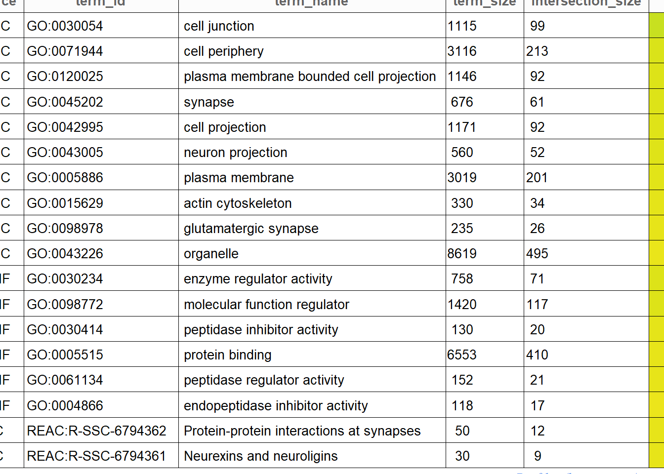
Figure 5.15: Gene Ontology enrichment table for the entire group of genotyped pigs.