6 Regression
Regression analysis will likely be the main focal
6.1 Linear Models
The basic linear regression function in R is lm, which performs OLS regression. The lm function, like most model functions, requires two elements to get started - a formula and data. The formula for the model is in the form you are used to for OLS, such that \(y = X_i \beta + \epsilon_i\) is equivalent to y ~ x. Data is given by data = data and is usually in the form of a data frame. Let’s look at an example.
data("mtcars")

model <- lm(mpg ~ disp, data = mtcars)
summary(model)
##
## Call:
## lm(formula = mpg ~ disp, data = mtcars)
##
## Residuals:
## Min 1Q Median 3Q Max
## -4.8922 -2.2022 -0.9631 1.6272 7.2305
##
## Coefficients:
## Estimate Std. Error t value Pr(>|t|)
## (Intercept) 29.599855 1.229720 24.070 < 2e-16 ***
## disp -0.041215 0.004712 -8.747 9.38e-10 ***
## ---
## Signif. codes: 0 '***' 0.001 '**' 0.01 '*' 0.05 '.' 0.1 ' ' 1
##
## Residual standard error: 3.251 on 30 degrees of freedom
## Multiple R-squared: 0.7183, Adjusted R-squared: 0.709
## F-statistic: 76.51 on 1 and 30 DF, p-value: 9.38e-10plot(mtcars$disp, mtcars$mpg)
abline(coef(model), col = "blue")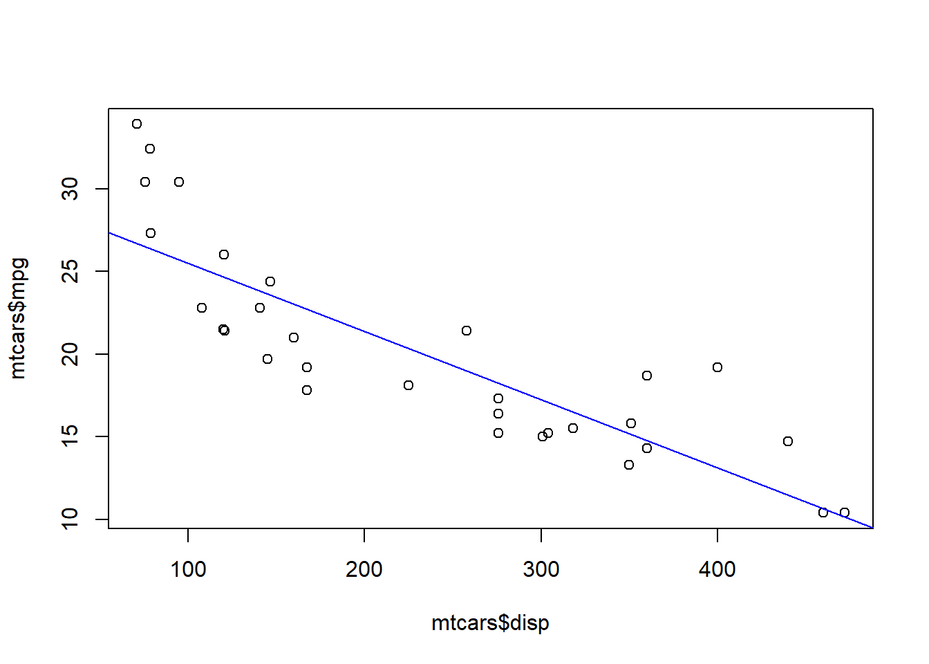
In mutivariate situation we are not able to plot the regression coefficients on a single plot. However we can plot them using the car package function avPlots to view the marginals for each explanatory variable.
model2 <- lm(mpg ~ disp + cyl + wt + drat, data = mtcars)
summary(model2)
##
## Call:
## lm(formula = mpg ~ disp + cyl + wt + drat, data = mtcars)
##
## Residuals:
## Min 1Q Median 3Q Max
## -4.4067 -1.4096 -0.4954 1.3346 6.0729
##
## Coefficients:
## Estimate Std. Error t value Pr(>|t|)
## (Intercept) 41.160271 7.304325 5.635 5.56e-06 ***
## disp 0.007472 0.012062 0.619 0.54080
## cyl -1.786074 0.634821 -2.814 0.00903 **
## wt -3.638075 1.102460 -3.300 0.00272 **
## drat -0.010492 1.337929 -0.008 0.99380
## ---
## Signif. codes: 0 '***' 0.001 '**' 0.01 '*' 0.05 '.' 0.1 ' ' 1
##
## Residual standard error: 2.642 on 27 degrees of freedom
## Multiple R-squared: 0.8326, Adjusted R-squared: 0.8078
## F-statistic: 33.57 on 4 and 27 DF, p-value: 4.057e-10library(car)
avPlots(model2)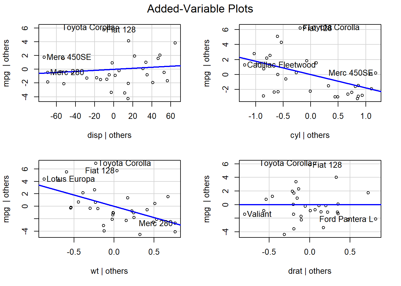
6.2 Logistic Regression
To perform logistic regression in R we will focus on the “general linear model” function which follows from the class of models by the same name. This function is imaginitively named glm and takes the same form as the OLS function lm. In this example we will model a binary outcome variable using the logit link function.
mtcars.bin <- mtcars
mtcars.bin$mpg <- 1*(mtcars.bin$mpg > 21)

model3 <- glm(mpg ~ disp + cyl + wt + drat, data = mtcars.bin,
              family = binomial(link = "logit"))
summary(model3)
##
## Call:
## glm(formula = mpg ~ disp + cyl + wt + drat, family = binomial(link = "logit"),
## data = mtcars.bin)
##
## Deviance Residuals:
## Min 1Q Median 3Q Max
## -1.866e-05 -2.110e-08 -2.110e-08 2.110e-08 2.292e-05
##
## Coefficients:
## Estimate Std. Error z value Pr(>|z|)
## (Intercept) 3.469e+02 1.544e+06 0.000 1
## disp 9.035e-01 1.490e+03 0.001 1
## cyl -7.122e+01 2.026e+05 0.000 1
## wt -4.885e+01 4.645e+05 0.000 1
## drat 8.582e+00 3.189e+05 0.000 1
##
## (Dispersion parameter for binomial family taken to be 1)
##
## Null deviance: 4.2340e+01 on 31 degrees of freedom
## Residual deviance: 1.1643e-09 on 27 degrees of freedom
## AIC: 10
##
## Number of Fisher Scoring iterations: 25Prediction and confusion matrix
pred3.bin <- data.frame(
  mpg = mtcars.bin$mpg,
  mpg.pred = predict(model3, newdata = mtcars.bin, type = "response")
)

pred3.bin$mpg.bin <- 1*(pred3.bin$mpg.pred > 0.5)

library(caret)
confusionMatrix(factor(pred3.bin$mpg), factor(pred3.bin$mpg.bin))
## Confusion Matrix and Statistics
##
## Reference
## Prediction 0 1
## 0 20 0
## 1 0 12
##
## Accuracy : 1
## 95% CI : (0.8911, 1)
## No Information Rate : 0.625
## P-Value [Acc > NIR] : 2.939e-07
##
## Kappa : 1
##
## Mcnemar's Test P-Value : NA
##
## Sensitivity : 1.000
## Specificity : 1.000
## Pos Pred Value : 1.000
## Neg Pred Value : 1.000
## Prevalence : 0.625
## Detection Rate : 0.625
## Detection Prevalence : 0.625
## Balanced Accuracy : 1.000
##
## 'Positive' Class : 0
## We can change our glm to match the data analysis we wish to perform by changing the family of the model. The family refers to the link function that R will use when performing the regression.
binomial(link="logit")guassian(link="identity")Gamma(link="inverse")poisson(link="log")quasi(link="identity", variance="constant")
6.3 Hypothesis Tests
one-way t-test
# some random data
x <- rnorm(100, 1, 0.5)

# t-test
t.test(x, mu=1.2)
##
## One Sample t-test
##
## data: x
## t = -4.2235, df = 99, p-value = 5.35e-05
## alternative hypothesis: true mean is not equal to 1.2
## 95 percent confidence interval:
## 0.9004436 1.0919413
## sample estimates:
## mean of x
## 0.9961925# directional
t.test(x, mu=1.2, alternative = "greater")##
## One Sample t-test
##
## data: x
## t = -4.2235, df = 99, p-value = 1
## alternative hypothesis: true mean is greater than 1.2
## 95 percent confidence interval:
## 0.9160699 Inf
## sample estimates:
## mean of x
## 0.9961925two-way t-test
# some random data
x <- rnorm(100, 1, 0.5)
y1 <- rnorm(100, 0, 1.2)
y2 <- rnorm(100, 1, 0.5)

# note difference in p-value
t.test(x, y1)
##
## Welch Two Sample t-test
##
## data: x and y1
## t = 9.185, df = 134.41, p-value = 6.618e-16
## alternative hypothesis: true difference in means is not equal to 0
## 95 percent confidence interval:
## 0.8861011 1.3724189
## sample estimates:
## mean of x mean of y
## 1.0044594 -0.1248007t.test(x, y2)##
## Welch Two Sample t-test
##
## data: x and y2
## t = 0.081147, df = 197.97, p-value = 0.9354
## alternative hypothesis: true difference in means is not equal to 0
## 95 percent confidence interval:
## -0.1290327 0.1401076
## sample estimates:
## mean of x mean of y
## 1.0044594 0.9989219Other tests:
- Wilcox - used when data is non-parametric
- Correlation - used when you want to compare the correlation between two variables
# some random data
x <- rnorm(100, 1, 0.5)
y <- rnorm(100, 0, 1.2)

wilcox.test(x, y)
##
## Wilcoxon rank sum test with continuity correction
##
## data: x and y
## W = 7917, p-value = 1.032e-12
## alternative hypothesis: true location shift is not equal to 0cor.test(x, y)##
## Pearson's product-moment correlation
##
## data: x and y
## t = -0.4892, df = 98, p-value = 0.6258
## alternative hypothesis: true correlation is not equal to 0
## 95 percent confidence interval:
## -0.2434145 0.1485016
## sample estimates:
## cor
## -0.049356126.4 Nonlinear Models
The built-in function nls is used to find parameter values of non-linear models in R. Non-linear models take the generic form \(y = f(x, \beta)\), where \(y\) is a set of outcome variables, \(x\) represents a set of random variables, and \(\beta\) represents the parameters of the model, such that \(f(x, \beta)\) cannot be expressed as a linear combination of the \(\beta\).
from RPubs - https://rpubs.com/RobinLovelace/nls-function
len <- 24
x = runif(len)
y = x^3 + runif(len, min = -0.1, max = 0.1)
plot(x, y)
s <- seq(from = 0, to = 1, length = 50)
lines(s, s^3, lty = 2)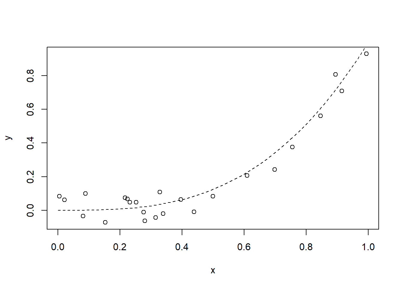
df <- data.frame(x, y)
m <- nls(y ~ I(x^power), data = df, start = list(power = 1), trace = T)
## 1.830568 (2.11e+00): par = (1)
## 0.4111573 (1.69e+00): par = (1.884938)
## 0.1150580 (5.84e-01): par = (2.832978)
## 0.08663172 (5.39e-02): par = (3.369605)
## 0.08639049 (1.44e-03): par = (3.432622)
## 0.08639032 (5.82e-05): par = (3.4309)
## 0.08639032 (2.33e-06): par = (3.43097)6.5 Other Model Types
There are obviously hundreds of model types available to fit the analysis you are using in your research. There are too many to list here but I will give a few highlights to point you in the right direction for commonly used model types in the social sciences.
Mixed and Random Effects Models - using the package lme4 you will be able to create mixed and random effects models in R. The function call for this is lmer. A great resource for this can be found here: https://m-clark.github.io/mixed-models-with-R/ .
Ordinal data - If your data has an ordered structure the function ordinal will perform ordinal regression and can be used to analyze this type of data.