7 Data Manipulation
The techniques and processes needed to manipulate, clean, explore, and prepare data prior to analysis are among the most necessary for your career. For quantitative scholars these skills are paramount and often time will present greater challenges and require more time than the actual analysis itself. For qualitative scholars the innumerable data forms used my non-quantitative methods will require extensive use of data manipulation and cleaning techniques.
In this chapter we will explore cover core R functions that will be a mainstay in your data manipulation repertoire. I will also cover functions found in the dplyr package that will allow you to manipulate and explore data quickly and efficiently. I will then work through a data set — cleaning, exploring, and preparing — the data for analysis and replication.
7.1 Core Functions
The core functions you are most likely to use on a near daily basis are relate to the structure, names, type, and ordering of your data. These are:
names— refers to the variable names of a data framelevels— levels refers to the different elements contained within a factor variablestr— provides a print out of the structure of the data setsummary— summarizes the data setfactor— creates a factor type element of your dataas...— changes the data type or refers to the data type of a data elementc()— generates a listsample— generates a random sampleorder— orders a data elementcomplete.cases— removesNAfrom a data elementduplicated— removes duplicates from a data element
Using the mtcars data set, lets look at each of these.
set.seed(376)
data("mtcars")

## Look at the names, structure, and levels for a factored variable
names(mtcars)
## [1] "mpg" "cyl" "disp" "hp" "drat" "wt" "qsec" "vs" "am" "gear"
## [11] "carb"str(mtcars)## 'data.frame': 32 obs. of 11 variables:
## $ mpg : num 21 21 22.8 21.4 18.7 18.1 14.3 24.4 22.8 19.2 ...
## $ cyl : num 6 6 4 6 8 6 8 4 4 6 ...
## $ disp: num 160 160 108 258 360 ...
## $ hp : num 110 110 93 110 175 105 245 62 95 123 ...
## $ drat: num 3.9 3.9 3.85 3.08 3.15 2.76 3.21 3.69 3.92 3.92 ...
## $ wt : num 2.62 2.88 2.32 3.21 3.44 ...
## $ qsec: num 16.5 17 18.6 19.4 17 ...
## $ vs : num 0 0 1 1 0 1 0 1 1 1 ...
## $ am : num 1 1 1 0 0 0 0 0 0 0 ...
## $ gear: num 4 4 4 3 3 3 3 4 4 4 ...
## $ carb: num 4 4 1 1 2 1 4 2 2 4 ...levels(factor(mtcars$cyl))## [1] "4" "6" "8"## Create a factor variable
## change the name of that variable
## create new numeric variable
mtcars$cyl <- factor(mtcars$cyl)
names(mtcars)[2] <- c("f.cyl")
mtcars$cyl <- as.numeric(mtcars$f.cyl)
## Sample 10 rows from the data set
## order the data by mpg ascending
## generate some NAs in the data
s.mtcars <- mtcars[sample(nrow(mtcars), 10, replace = FALSE), c(1:4)]
s.mtcars <- s.mtcars[order(s.mtcars$mpg), ]
.tmp. <- as.character(s.mtcars$f.cyl)
.tmp.[ .tmp. == "6" ] <- NA
s.mtcars$f.cyl <- factor(.tmp.)
s.mtcars## mpg f.cyl disp hp
## Camaro Z28 13.3 8 350.0 245
## Ford Pantera L 15.8 8 351.0 264
## Merc 450SE 16.4 8 275.8 180
## Merc 450SL 17.3 8 275.8 180
## Hornet Sportabout 18.7 8 360.0 175
## Merc 280 19.2 <NA> 167.6 123
## Mazda RX4 Wag 21.0 <NA> 160.0 110
## Hornet 4 Drive 21.4 <NA> 258.0 110
## Merc 230 22.8 4 140.8 95
## Lotus Europa 30.4 4 95.1 113## Remove rows that have NAs from the f.cyl variable
## Remove rows that have duplicate values in disp and hp
s.mtcars <- s.mtcars[complete.cases(s.mtcars$f.cyl), ]
s.mtcars <- s.mtcars[!duplicated(s.mtcars[,c(3:4)]), ]
s.mtcars## mpg f.cyl disp hp
## Camaro Z28 13.3 8 350.0 245
## Ford Pantera L 15.8 8 351.0 264
## Merc 450SE 16.4 8 275.8 180
## Hornet Sportabout 18.7 8 360.0 175
## Merc 230 22.8 4 140.8 95
## Lotus Europa 30.4 4 95.1 1137.1.1 Apply Functions
There are 4 apply functions in R. These functions allow you to avoid writing explicit loops to manipulate or translate your data. Note: many package functions such as the substr function in the next section make use of the apply functions in their source code, and therefore when using these non-base function, the apply functions are superfluous.
apply The apply function takes three inputs: the data, the ‘margin’, and the function you wish to ‘apply’. For the apply function, the margin references how the function should be applied: 1 = by row, 2 = by column, or c(1,2) by both row and column. The function you are trying to apply can be any base or user defined function so long as it makes sense to use the function on a vector contained in a data frame or matrix.
m <- matrix(runif(25), nrow = 5, ncol = 5)
m
## [,1] [,2] [,3] [,4] [,5]
## [1,] 0.7440106 0.40818452 0.3236927 0.62695652 0.8126530
## [2,] 0.3986270 0.14580755 0.2285263 0.04535837 0.6395984
## [3,] 0.5301235 0.45755373 0.7419694 0.24907242 0.6248807
## [4,] 0.8655568 0.09325418 0.4980100 0.65967279 0.4101029
## [5,] 0.9123481 0.09381158 0.5071449 0.60856733 0.6166991m.a <- apply(m, 1, mean)
m.a## [1] 0.5830995 0.2915835 0.5207200 0.5053193 0.5477142lapply The lapply function takes as its input a list and returns a list after applying the called function to each element in the list — hence the ‘l’ for list.
l <- c('99', 'problems', 'but', 'a', 'dataset', 'aint', 'one')

l.a <- lapply(l, toupper) # upper case all words
l.a <- unlist(l.a) # unlist l.a element
str(l.a) # print structure
## chr [1:7] "99" "PROBLEMS" "BUT" "A" "DATASET" "AINT" "ONE"sapply The sapply function acts in the same way as the lapply function but instead of working on lists and returning a list, the sapply function returns a vector or matrix and works on data frames as well. To show this will work with a user defined function, let’s take the normalize function from chapter 4 and try to apply it to all elements of a data frame.
# Normalization function
normalizeMe <- function(x){
  n <- (x - min(x))/(max(x) - min(x))
  return(n)
}

# Make data frame
df <- data.frame(v1 = exp(runif(100)*2), v2 = rnorm(100, 5, 2.3))
plot(df$v1, df$v2)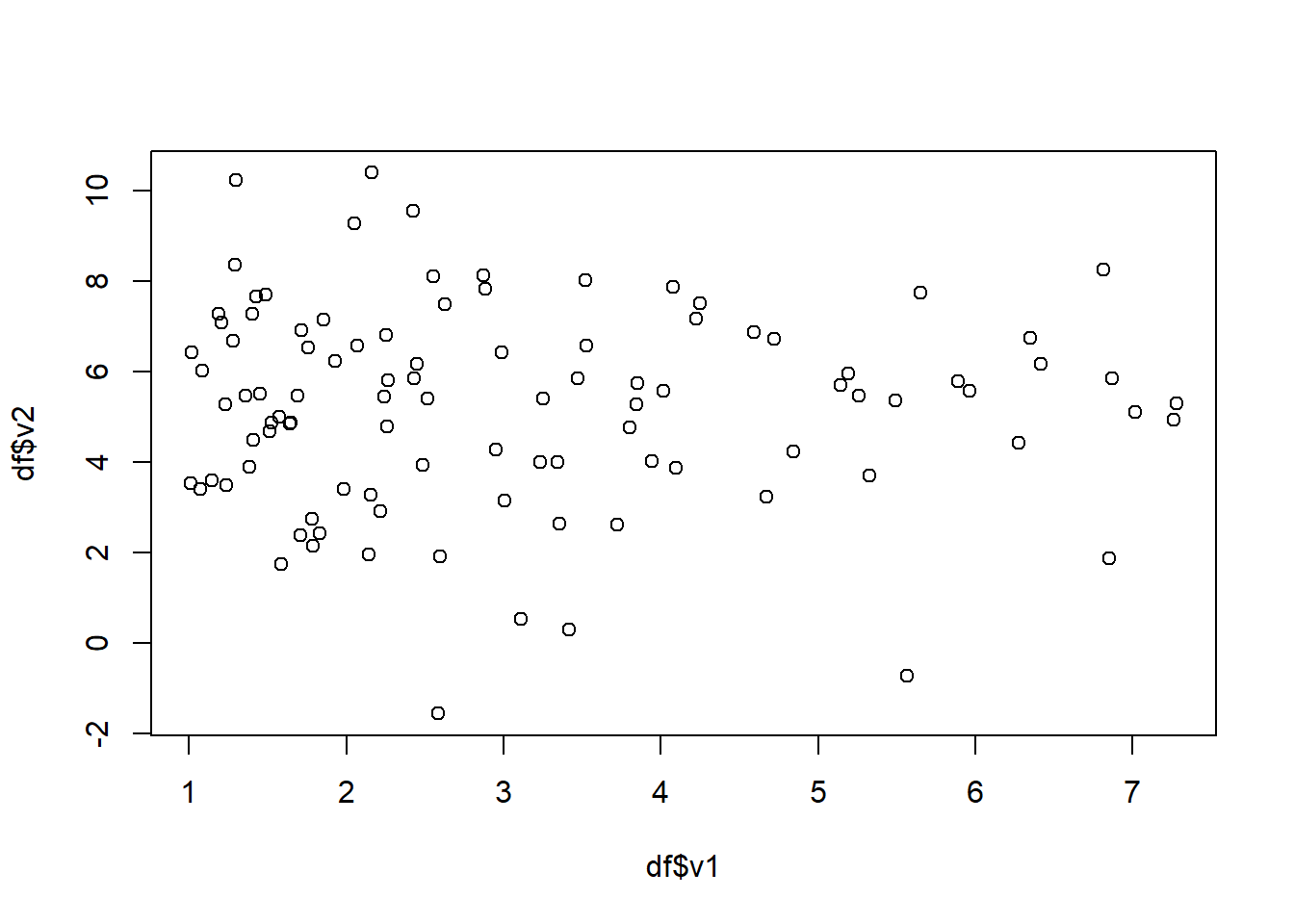
# Use sapply to normalize df$test
norm.df <- as.data.frame(sapply(df, normalizeMe))
plot(norm.df$v1, norm.df$v2)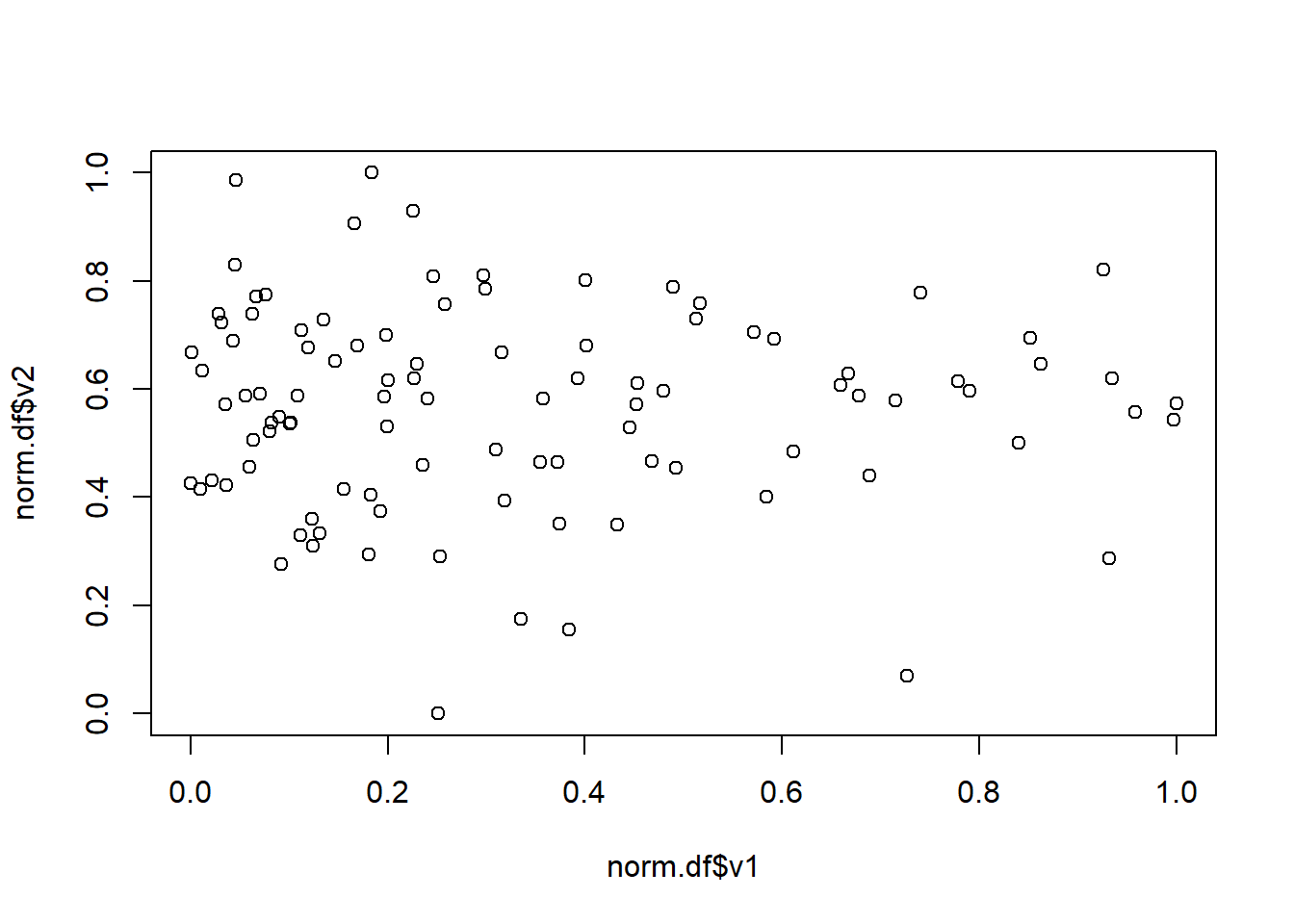
tapply The tapply function is a bit different from the other three and is maybe a bit less useful given your familiarity with dplyr. However, the speed of the tapply function is unmatched for large data sets. This function takes three main inputs: a vector to apply some function, a factor to group by, the function to apply by group to the vector. Using the chickwts data set, we have weights (a numeric vector) of chicks by feed type (a factor vector). Here we find the mean of chick weights by feed type.
data("chickwts")
str(chickwts)
## 'data.frame': 71 obs. of 2 variables:
## $ weight: num 179 160 136 227 217 168 108 124 143 140 ...
## $ feed : Factor w/ 6 levels "casein","horsebean",..: 2 2 2 2 2 2 2 2 2 2 ...tapply(chickwts$weight, chickwts$feed, mean)## casein horsebean linseed meatmeal soybean sunflower
## 323.5833 160.2000 218.7500 276.9091 246.4286 328.91677.1.2 Dates and Strings
There are two additional elements that will show up in your data often that require data manipulation — dates and partial variables. There are two main types of dates in R, as.Date and POSIX dates. Sometimes it is necessary to work with both types while doing your data manipulation; however, I think in general it is easier to create POSIX dates if you find yourself working with dates a lot. A useful website for dates is: https://www.stat.berkeley.edu/~s133/dates.html
## as.Date function
dates <- c("2022/10/17","2022/10/16","2022/10/15")
dates <- as.Date(dates, format = '%Y/%m/%d')
str(dates)
## Date[1:3], format: "2022-10-17" "2022-10-16" "2022-10-15"## POSIX dates
dates <- as.POSIXct(dates) # create POSIX date element
dates <- dates + (3600*rnorm(3)) # add noise to the time stamp
str(dates)## POSIXct[1:3], format: "2022-10-16 19:56:57" "2022-10-15 16:51:30" "2022-10-14 19:19:31"The need to get a specific part of a data element will also arise often. Unfortunately for the beginner, there are several ways to accomplish this task. The grep functions are the most powerful and ultimately the most broadly useful, but are difficult and unintuitive. A more intuitive way of thinking about selecting a portion of an element is to think of the element as a string from which you want a part of that string. This is referred to as a substring and can be very useful when manipulating or analyzing data.
library(stringr) # useful package

l <- c('99', 'problems', 'but', 'a', 'dataset', 'aint', 'one')
l <- str_pad(l, 10, side="right", pad="x")
l <- substr(l, 1, 5)
l
## [1] "99xxx" "probl" "butxx" "axxxx" "datas" "aintx" "onexx"7.2 Dplyr Functions
The dplyr package as we have previously discussed is very powerful. In this section I will give a brief overview of the ways in which dplyr can be used to modify and analyze data. Note the dplyr package makes use of a cool control element for your code - the ‘pipe’ written as %>%.
Part 1: These are the functions that you will use most often in dplyr.
filtergroup_bysummariseleft_join
library(dplyr)

data("mtcars")
df <- mtcars

## Filter data frame df
## Group summary by a factor of the variable cyl
## Summarize 4 additional variables: 3 mean, 1 max
df %>%
  filter(mpg >= 20 | hp >= 100) %>%
  group_by(factor(cyl)) %>%
  summarise(meanDisp = mean(disp),
            meanHP = mean(hp),
            meanWt = mean(wt),
            maxGear = max(gear))
## # A tibble: 3 x 5
## `factor(cyl)` meanDisp meanHP meanWt maxGear
## <fct> <dbl> <dbl> <dbl> <dbl>
## 1 4 105. 82.6 2.29 5
## 2 6 183. 122. 3.12 5
## 3 8 353. 209. 4.00 5## Create extraneous table to join
dt <- data.frame(CarName = factor(row.names(df)),
Cylinders = df$cyl,
Horsepower = df$hp,
RandomVar = rbeta(nrow(df), 0.8, 0.5))
## Join the extraneous table to the data frame
## Remove duplicate entries created by join
df2 <- left_join(df, dt, by=c("cyl" = "Cylinders", "hp" = "Horsepower"))
df2 <- df2[!duplicated(df2$CarName),]
str(df2)## 'data.frame': 32 obs. of 13 variables:
## $ mpg : num 21 21 21 22.8 18.7 18.7 18.1 14.3 14.3 24.4 ...
## $ cyl : num 6 6 6 4 8 8 6 8 8 4 ...
## $ disp : num 160 160 160 108 360 ...
## $ hp : num 110 110 110 93 175 175 105 245 245 62 ...
## $ drat : num 3.9 3.9 3.9 3.85 3.15 3.15 2.76 3.21 3.21 3.69 ...
## $ wt : num 2.62 2.62 2.62 2.32 3.44 3.44 3.46 3.57 3.57 3.19 ...
## $ qsec : num 16.5 16.5 16.5 18.6 17 ...
## $ vs : num 0 0 0 1 0 0 1 0 0 1 ...
## $ am : num 1 1 1 1 0 0 0 0 0 0 ...
## $ gear : num 4 4 4 4 3 3 3 3 3 4 ...
## $ carb : num 4 4 4 1 2 2 1 4 4 2 ...
## $ CarName : Factor w/ 32 levels "AMC Javelin",..: 18 19 13 5 14 27 31 7 3 21 ...
## $ RandomVar: num 0.872 0.988 0.86 0.403 0.771 ...Part 2: These functions are the core functions of dyplr but I find they get used less often that the above.
arrangemutateselectslice
## Order the data descending by mpg, ascending by disp
df %>%
  filter(mpg >= 22) %>%
  arrange(desc(mpg), disp)
## mpg cyl disp hp drat wt qsec vs am gear carb
## Toyota Corolla 33.9 4 71.1 65 4.22 1.835 19.90 1 1 4 1
## Fiat 128 32.4 4 78.7 66 4.08 2.200 19.47 1 1 4 1
## Honda Civic 30.4 4 75.7 52 4.93 1.615 18.52 1 1 4 2
## Lotus Europa 30.4 4 95.1 113 3.77 1.513 16.90 1 1 5 2
## Fiat X1-9 27.3 4 79.0 66 4.08 1.935 18.90 1 1 4 1
## Porsche 914-2 26.0 4 120.3 91 4.43 2.140 16.70 0 1 5 2
## Merc 240D 24.4 4 146.7 62 3.69 3.190 20.00 1 0 4 2
## Datsun 710 22.8 4 108.0 93 3.85 2.320 18.61 1 1 4 1
## Merc 230 22.8 4 140.8 95 3.92 3.150 22.90 1 0 4 2## Slice selection the 7th through 14th rows
df %>%
slice(7:13)## mpg cyl disp hp drat wt qsec vs am gear carb
## Duster 360 14.3 8 360.0 245 3.21 3.57 15.84 0 0 3 4
## Merc 240D 24.4 4 146.7 62 3.69 3.19 20.00 1 0 4 2
## Merc 230 22.8 4 140.8 95 3.92 3.15 22.90 1 0 4 2
## Merc 280 19.2 6 167.6 123 3.92 3.44 18.30 1 0 4 4
## Merc 280C 17.8 6 167.6 123 3.92 3.44 18.90 1 0 4 4
## Merc 450SE 16.4 8 275.8 180 3.07 4.07 17.40 0 0 3 3
## Merc 450SL 17.3 8 275.8 180 3.07 3.73 17.60 0 0 3 3## Slice a sample of 10 rows and order by mpg
df %>%
slice_sample(n = 10) %>%
arrange(mpg)## mpg cyl disp hp drat wt qsec vs am gear carb
## Lincoln Continental 10.4 8 460.0 215 3.00 5.424 17.82 0 0 3 4
## Cadillac Fleetwood 10.4 8 472.0 205 2.93 5.250 17.98 0 0 3 4
## Maserati Bora 15.0 8 301.0 335 3.54 3.570 14.60 0 1 5 8
## Merc 280C 17.8 6 167.6 123 3.92 3.440 18.90 1 0 4 4
## Valiant 18.1 6 225.0 105 2.76 3.460 20.22 1 0 3 1
## Pontiac Firebird 19.2 8 400.0 175 3.08 3.845 17.05 0 0 3 2
## Hornet 4 Drive 21.4 6 258.0 110 3.08 3.215 19.44 1 0 3 1
## Merc 230 22.8 4 140.8 95 3.92 3.150 22.90 1 0 4 2
## Porsche 914-2 26.0 4 120.3 91 4.43 2.140 16.70 0 1 5 2
## Toyota Corolla 33.9 4 71.1 65 4.22 1.835 19.90 1 1 4 1## Select specific columns from the df
df %>%
select(mpg, disp, hp) %>%
slice_head(n = 3)## mpg disp hp
## Mazda RX4 21.0 160 110
## Mazda RX4 Wag 21.0 160 110
## Datsun 710 22.8 108 93## Mutate to add a column that is mpg / hp
df %>%
mutate(mpg.hp = mpg/hp) %>%
select(mpg.hp, mpg, hp) %>%
slice_max(mpg.hp)## mpg.hp mpg hp
## Honda Civic 0.5846154 30.4 52There are lots of good references out there for dplyr including the main CRAN vignette: https://cran.r-project.org/web/packages/dplyr/vignettes/dplyr.html