4 Loops and Functions

For loops and functions form the core of the skills you will need to solve many of your programming challenges in R.

Loop — A loop is what is sounds like, such that when programming a ‘loop’ you are telling the computer to recursively iterate through a set of steps outlined within the loop.

• Loops can contain functions, calls to data, create data, and contain other ‘nested’ loops.
• In R a ‘for loop’ begins with the syntax for(){} such that the user specifies the concept of iteration in the () and the steps within the loop {}.
• Loops are useful for solving all types of programming and statistical problems, such as iterative ifelse statements, decomposing data, and serving helper functions over wide datas ets.
• Loops in R are resource intensive and slow comparatively to other programming languages (like C++), and this computational speed should be considered when writing complicated for loops.

Function — A function can be thought of as a self contained ‘program’ of sorts. A function takes an input and performs the operations defined in the function on the input, returning the output to the user.

• A function can contain other functions, loops, and complex logic.
• To call a function, the syntax in R is always the same — functionName().
• Base R and R’s various libraries can be thought of as generally consisting of ‘functions’ — for example, the caret package contains the train() function used to perform various machine learning modeling tasks.
• When considering if you need to write your own function answer the question - ‘Will I need to use this code, in the same way, many times?’ - If the answer is yes, then you should write a function, if the answer is no, then you could write your own function, but it may not be necessary to do so.

4.1 Loops

Basic loops:

— The following syntax shows the basic structure of a for loop in R. In this loop we iterate 5 times with our iteration index i serving as the input for our treatment of the created variable x. We then print the output of the loop at each iteration.

for(i in 1:5){
  x <- i^2 
  print(x)
}

## [1] 1
## [1] 4
## [1] 9
## [1] 16
## [1] 25

Loops inside loops:

— These are nested for loops, such that for each iteration of the outer loop, the inner loop completes a full cycle of its specified iteration count.

# set p
p <- c()

for(i in 1:20){
  x <- log(i)
  
  for(j in 1:10){
    y <- (x * j)
    p <- rbind(p, y)
  }
  
  ifelse(i > 15, print(i), NA)
}

## [1] 16
## [1] 17
## [1] 18
## [1] 19
## [1] 20

plot(p)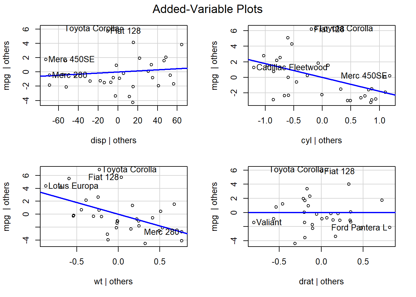

Value loops:

— A ‘value’ loop is a for loop that instead of iterating through a sequence of numbers instead iterates through a series of ‘string’ values.

# Create list names you want loop through
namestoloop <- names(df[3:25])
coefs <- c()

for(value in namestoloop){
  form <- as.formula(paste(value, "~ x1", sep = " "))
  fit <- lm(form, data=df)
  beta <- fit$coefficients
  coefs <- rbind(coefs, beta)
}

4.2 Functions

Single-line function:

— A single-line function is a syntax in R where you can write a function on a single line without the bracket syntax of a multi-line function. Here we create the Sigmoid function, \(S = \frac{1}{1+e^{-x}}\), in a single line.

singleLine.func <- function(x) 1/(1 + exp(1)^(-x))
singleLine.func(5)

## [1] 0.9933071

Multi-Line function:

— A multi-line function follows the syntax functionName(input){operation return} and is how you will generally write most functions. In this silly example, we take three inputs, create an Gaussian \(\epsilon\) term, perform an algebraic function on the variable y and return y for the set of all inputs.

set.seed(1234)

multiLine.func <- function(x, beta, lambda){
  epsilon <- rnorm(1)
  y = x*beta + lambda + epsilon
  return(y)
}

x <- runif(50)*10
beta <- rbeta(50, 5, 2)
lambda <- rnorm(50)

out.y <- multiLine.func(x, beta, lambda)
plot(out.y)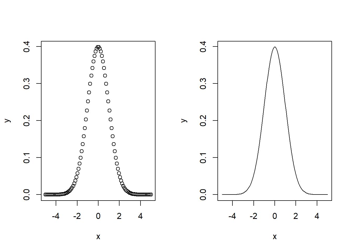

We can also use a function to transform another function — such as using our single and multiple line functions together

plot(
  singleLine.func(
    multiLine.func(x, beta, lambda)
    ),
  ylab = "sigmoid_y")

4.2.1 Helper Functions

Another way to use functions in R is to create ‘helper’ type functions. These functions perform a simple, computationally inexpensive tasks that you typically will use while doing more complex tasks. Examples of helper functions are the normalization and standardization functions below perform a mathematical operation on data. Other helper function such as Euclidean Distance or Great Circle perform a specific calculation from data. The difference between these types of helper functions is what we want from the input — e.g. do we want to transform the input or do we want to know something from the input. A third type of function, such as a Binary Gap function tells us something about our data. In any case, understanding what we want from our data before writing your function is essential.

Normalization function: \(N = \frac{X - X_{min}}{X_{max} - X_{min}}\)

normalizeMe <- function(x){
  n <- (x - min(x))/(max(x) - min(x))
  return(n)
}

norm.y <- normalizeMe(out.y)
plot(norm.y)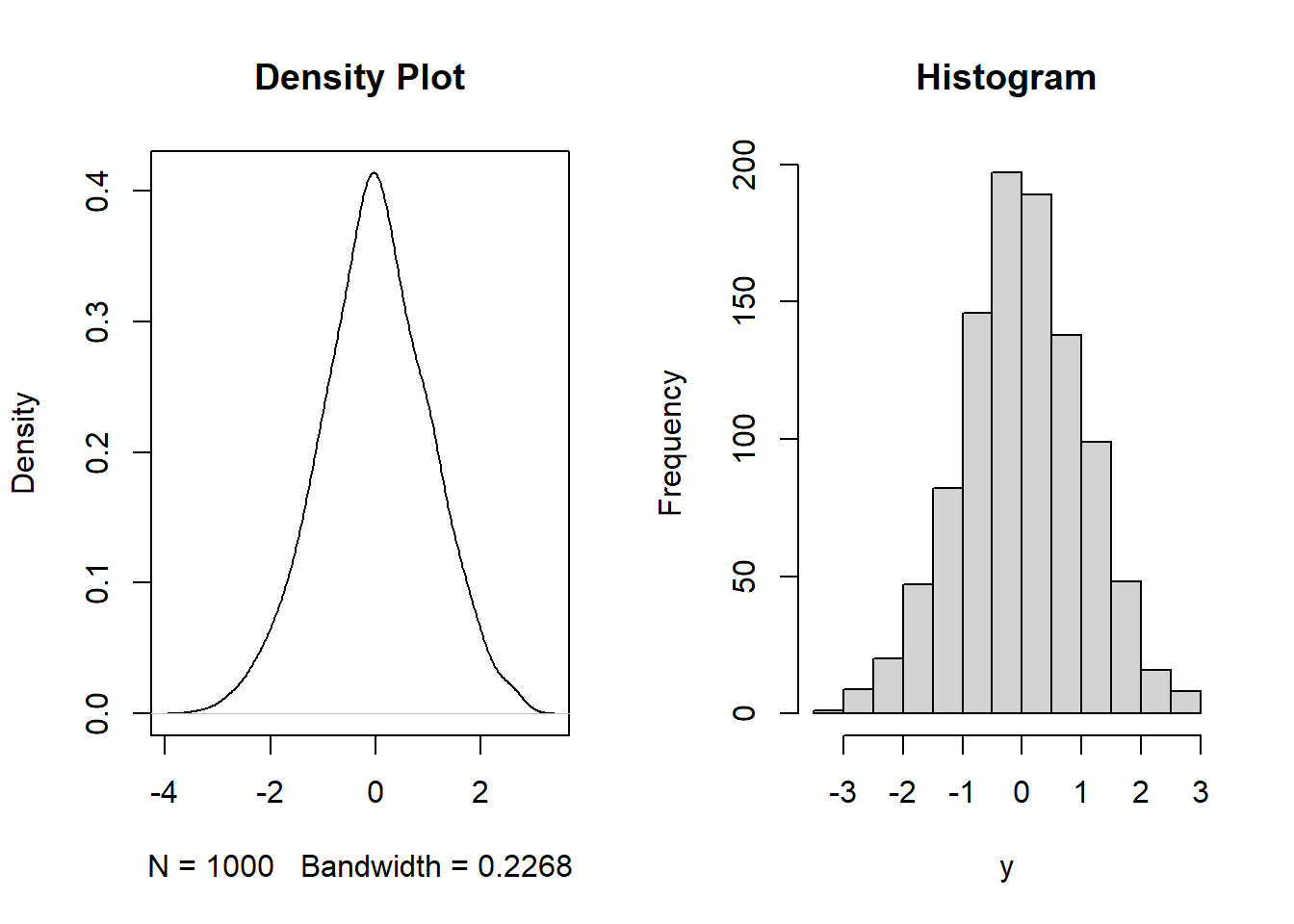

Standardization Function: \(s = \frac{x-\mu}{\sigma}\)

standardizeMe <- function(x){
  mu <- mean(x)
  sigma <- sd(x)
  s <- (x - mu)/sigma
  return(s)
}

stand.y <- standardizeMe(out.y)
plot(stand.y)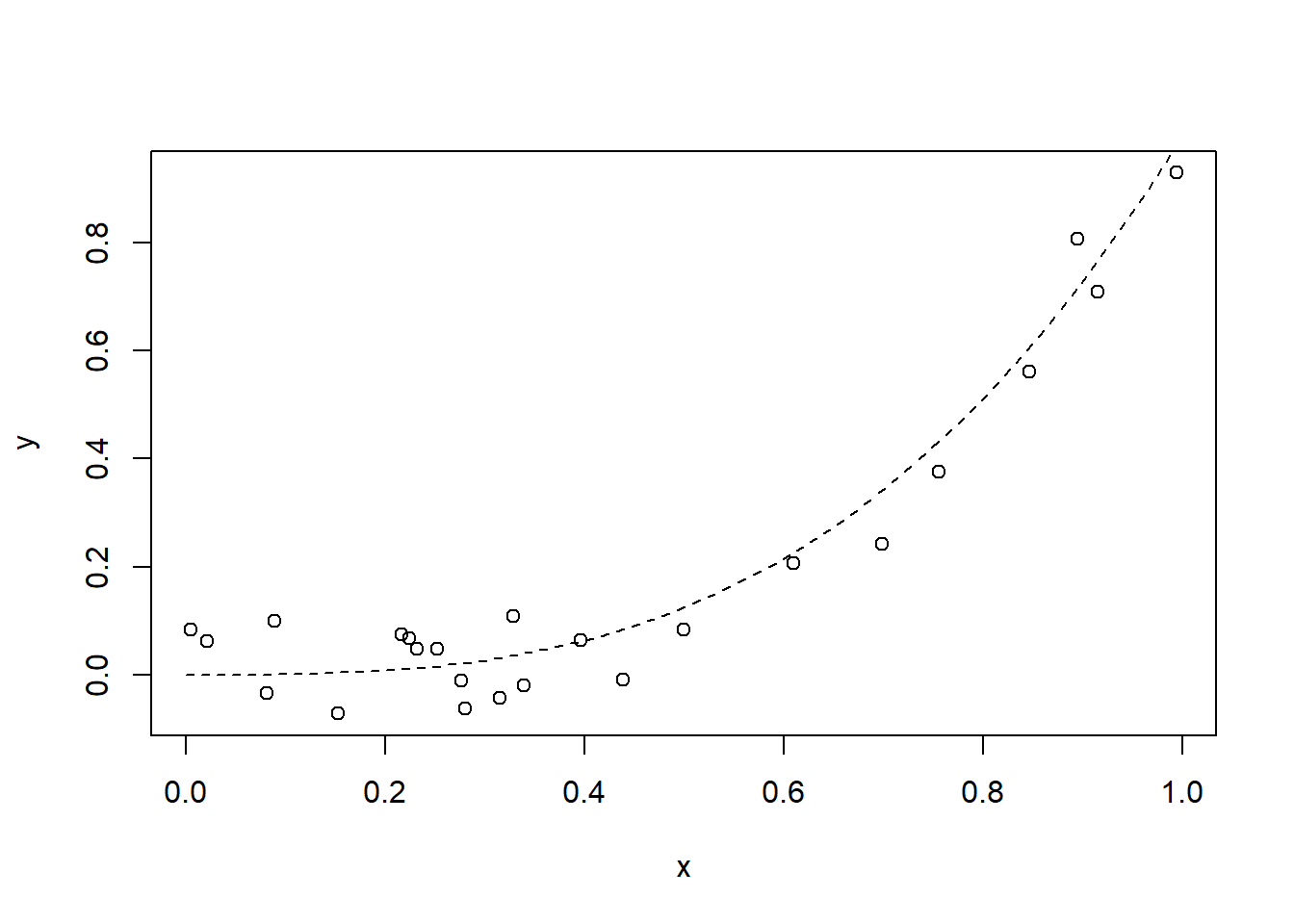

4.2.2 Functional Programming

Functional programming is a map of values to other values and is declarative, meaning you are telling the computer the logic you want it to perform. Functional Programming separates the logic from the data, unlike object oriented programming - where an object is an abstraction of logic and data. R functions, are fundamentally a functional programming style.

4.3 Data Manipulation

Unlist a column of type list in a data frame:

• df = a data frame
• idVar = identification variable
• listVar = a column in the data frame with a list of data nested at each row

fill.df <- data.frame()
out <- c()
nscan <- nrow(df)

for(i in 1:nscan){
  id <- df$idVar[i]
  
  V1 <- df$listVar[[i]][1] # the first element of the list in the i'th row
  V2 <- df$listVar[[i]][2] # the second element of the list in the i'th row
  V3 <- df$listVar[[i]][3]
  ...
  Vk <- df$listVar[[nrow]][k] # the k'th element of the list in the n'th row
  
  out <- cbind(id, V1, V2, V3, ..., Vk)
  filt.df <- rbind(fill.df, out)
}

Of course it is easier to just write…

  listVar <- df$listVar
  listMerge <- as.data.frame(t(sapply(listVar, `length<-`, max(lengths(listVar)))))
  listMerge$id = df$id
  dfSanListVar <- merge(df[,-c("listVar")], listMerge, by="id")

… But you get the idea. Loops can be use to do any sort of iterative task.

4.4 Example Code

Binary Gap Function:

— Find the largest gap between 1’s in the binary string of a number.

N <- 275610687

binarygap <- function(Number){
  x <- as.integer(intToBits(Number))
  s <- c()
  m <- 0
  
  for(i in 1:31){
    if(x[i] + x[i+1] == 2){
      m <- 0
    } else if(x[i] + x[i+1] == 1){
      m <- 1
    } else if(x[i] + x[i+1] == 0){
      m <- m + 1
    }
    s <- rbind(s, m)
  }
  
  return(max(s))
}

print(as.integer(intToBits(N)))

##  [1] 1 1 1 1 1 1 0 0 0 0 1 1 1 1 1 0 1 0 1 1 0 1 1 0 0 0 0 0 1 0 0 0

binarygap(N)

## [1] 5

Gradient Decent Function:

— Perform gradient decent optimization to find the global minimum of a function.

# Make Gradient Descent Function
grad.des <- function(f, fprime, start, delta, alpha, precision, max.iters, verbose=FALSE){
  
  # Create Empty Sets
  x_list <- c()
  f_list <- c()
  fp <- c()
  n = 0
  x_0 = 0
  x_1 = start
  
  # While loop containing dual descent trajectories based on different alpha terms |
  # Trajectory 1 set by user for larger steps until algorithm approaches epsilon |
  # Trajectory 2 set by algorithm as alpha = 1/n until precision level reached |
  while(abs(fprime(x_0, delta)) >= precision & n <= max.iters-1){
    
    if(abs(fprime(x_0, delta)) >= 0.1){
      n <- n + 1
      
      x_0 <- x_1
      x_1 <- x_0 - alpha*fprime(x_0, delta)
    }
    else{
      n <- n + 1
      
      x_0 <- x_1
      x_1 <- x_0 - ((1/n)*fprime(x_0, delta))
    }
    
    x_list[[n]] <- x_1
    f_list[[n]] <- f(x_1)
    fp[[n]] <- fprime(x_0, delta)
    
  }
  
  gd.out <- list(N=n, x_star=x_list[[n]], f_star=f_list[[n]], fp_star=fp[[n]], 
                 x=x_list, f=f_list, fp=fp)
  return(gd.out)
  
}

# Random search of start points within values |
# User defines the size and scope of starting set |
# All options from the gradient descent algorithm are maintained |
rand.s <- function(lower.b, upper.b, size.b,
                   f, fprime, delta, alpha,
                   precision, max.iters, verbose=TRUE){
  
  # Random numbers generated inside user defined space
  d.search <- runif(size.b, min=lower.b, max=upper.b)
  
  fs.out <- data.frame()
  fs_list <- c()
  val_list <- c()
  
  # Loop over gradient descent function for values in random search |
  # Output is the minimum value for f(x) for each iteration and |
  # the start value for that iteration |
  for(value in d.search){
    
    gd.out <- grad.des(f=f, fprime=fprime, start=value, delta=delta, 
                       alpha=alpha, precision=precision, max.iters=max.iters)
    
    fs_list <- c(fs_list, gd.out$f_star)
    val_list <- c(val_list, value)
    
  }
  
  fs.out <- data.frame(startvalue=val_list, f_min=fs_list)
  return(fs.out)
}

# Random search function call
fs.out <- rand.s(lower.b=-2, upper.b=4, size.b=10000, f=f1, fprime=f.prime, 
                 delta=0.001, alpha=0.06, precision=0.05, max.iters=100, verbose=FALSE)

Loop Wrapper:

— Perform a Naive Bayes prediction model over 86 outcome variables.

wrapper_out <- data.frame(id = data_train$id)
namestoiterate <- names(data_train[,4:89])

for(i in 1:86){
  
  z1 <- paste(namestoiterate[i], "Var1", sep="~")
  mod_t <- as.formula(z1)
  fit_t <- bayesglm(mod_t, 
                    family = quasibinomial(link="logit"), 
                    data=data_train, 
                    weights = data_train$weight)
  x_t <- se.coef(fit_t)
  y_t <- sigma.hat(fit_t)
  notpred_t <- predict(fit_t, newdata=data_surv, type="response")
  prior_t <- data.frame( prior = notpred_t )
  
  z2 <- paste(namestoiterate[i], "Var1 + Var2 + Var3 + Var4 + Var5 + Var6", sep="~")
  p_t_mod <- as.formula(z2)
  p_t_fit <- bayesglm(p_t_mod, family = quasibinomial(link="logit"),
                      data = data_train,
                      prior.mean = mean(prior_t$prior, na.rm = TRUE),
                      prior.scale = y_t,
                      maxit = 1000, 
                      weights = data_train$weight)
  
  p_t <- data.frame(id = data_test$id, 
                    pred = predict(p_t_fit, newdata = data_test, type="response"))
  names(p_t)[2] <- namestoiterate[i]
  
  wrapper_out <- merge(wrapper_out, p_t, by="VUID")
  
}

Ising Model using a Gibbs Sampler:

nscan <- 1000 # number of iterations
# some square matrix of data that contains noise about the true image
y <- rbind(
  c( 1, 0, 0, 0, 1 ),
  c( 0, 1, 1, 1, 0 ),
  c( 0, 0, 1, 1, 0 ),
  c( 0, 1, 0, 0, 1 ),
  c( 1, 0, 0, 0, 1 ) )
kk <- nrow(y)  # number of rows/columns in matrix
x <- matrix(1,kk,kk) # an uninformative prior for the sampler to start from

# A Gibbs sampler (An MCMC algorithm)
phi <- 0.5 # tuning parameter
eps <- 0.1 # tuning parameter

pone <- matrix(0,kk,kk) # create placeholder for transition matrix
sumx <- numeric(nscan) # create placeholder to save value of x

# Ising Model in Gibbs Sampler
for( iscan in 1:nscan )
{
  for( i in 1:kk )
  {
    for( j in 1:kk )
    {
      # find relevant information from neighbors (nei)
      nei <- 0
      if( i>1 ){ nei <- nei + x[i-1,j] }
      if( i<kk ){ nei <- nei + x[i+1,j] }
      if( j>1 ){ nei <- nei + x[i,j-1] }
      if( j<kk ){ nei <- nei + x[i,j+1] }
      
      # Update by the simple full conditional (fc)
      fc.plus <- exp(phi*nei + y[i,j]*log(1-eps) + (1-y[i,j])*log(eps) )
      fc.minus <- exp(-phi*nei + y[i,j]*log(eps) + (1-y[i,j])*log(1-eps) )
      
      p <- fc.plus/(fc.plus+fc.minus)
      x[i,j] <- ifelse( runif(1) <= p, +1, -1 )
    }
    sumx[iscan] <- sum(x)
  }
  
  # update posterior mean approximation 
  pone <- pone + (x==1)/nscan
  print(iscan)
}