23 單變數迴歸
Lucky is he who has been able to understand the causes of things.
— Virgil (29 BC)
本部分將探討社會科學計量。本章為 Ismay and Kim (2019) 第 5 章內容。
需要的套件
library(tidyverse)
library(moderndive)
library(skimr)
library(gapminder)其中,moderndive 使用 tidyverse style 編寫,可以從事基本的線性迴歸;skimr 則可以幫助我們快速地計算敘述統計。
23.1 解釋變數為連續變數
以下,我們想了解的是老師的外貌與其教學評鑑的分數有關係嗎?是什麼關係?因此,解釋變數(explanatory variable) \(x\) 為老師的外貌分數,而結果變數(outcome variable)為老師的教學評鑑分數。
23.1.1 探索性資料分析
在 moderdive 中,有一 data frame 為 evals,其包含了 UT Austin 的 463 門課程。我們使用 select() 選取我們接下來將要使用的變數,包括 ID、score 與 bty_avg,並且存在名為 evals_ch5 裡頭。
evals_ch5 <- evals %>%
  select(ID, score, bty_avg)
回憶第 8 章所提及的,當我們拿到資料要分析或建模之前,第一件事情就是進行探索性資料分析,即 EDA。EDA 讓我們了解個別變數的分配、變數之間是否有潛在的關係與是否有 outliers 或缺漏值。EDA 常見的三個步驟:5
觀察原始資料的值。
計算概括的統計量,如平均數、中位數或四分位距等。
資料視覺化。
23.1.1.1 EDA:觀察原始資料的值
我們可以使用 tibble 中的 glimpse() 查看資料,如:
glimpse(evals_ch5)## Rows: 463
## Columns: 3
## $ ID <int> 1, 2, 3, 4, 5, 6, 7, 8, 9, 10, 11, 12, 13, 14, 15, 16, 17, 18,…
## $ score <dbl> 4.7, 4.1, 3.9, 4.8, 4.6, 4.3, 2.8, 4.1, 3.4, 4.5, 3.8, 4.5, 4.…
## $ bty_avg <dbl> 5.000, 5.000, 5.000, 5.000, 3.000, 3.000, 3.000, 3.333, 3.333,…也能使用 dplyr 中的 sample_n() 函數,隨機挑選給定數量的觀察值,如:
evals_ch5 %>%
  sample_n(size = 5)
## # A tibble: 5 × 3
## ID score bty_avg
## <int> <dbl> <dbl>
## 1 417 4.8 6.83
## 2 452 3.4 4.33
## 3 420 5 7.83
## 4 32 4.3 4.17
## 5 19 4.6 7.33由上,我們可知有 463 個觀察值。其中,各個變數分別代表:
ID:在這份資料中用以編號觀察值的變數。score:連續變數;老師的平均教學評鑑分數;最高 5 分,最低 1 分;為我們所關切的結果變數 \(y\)。bty_avg:連續變數;老師的平均外貌分數,最高 10 分,最低 1 分;為我們所關切的解釋變數 \(x\)。
23.1.1.2 EDA:簡單的敘述統計
既然 score 與 bty_avg 是連續的數值變數,那我們可以計算他們的平均值與中位數,如:
evals_ch5 %>%
  summarise(mean_score = mean(score),
            mean_bty_avg = mean(bty_avg),
            median_score = median(score),
            median_bty_avg = median(bty_avg))
## # A tibble: 1 × 4
## mean_score mean_bty_avg median_score median_bty_avg
## <dbl> <dbl> <dbl> <dbl>
## 1 4.17 4.42 4.3 4.33不過,如果要使用 summarize 來計算標準差、極值與分量的話,並非不可,只是比較麻煩。我們可以使用套件 skimr 中的 skim() 函數。把 data frame 丟入這個函數,將會回傳常用的敘述統計量,如:
evals_ch5 %>% select(score, bty_avg) %>% skim()── Data Summary ────────────────────────
Values
Name Piped data
Number of rows 463
Number of columns 2
_______________________
Column type frequency:
numeric 2
________________________
Group variables None
── Variable type: numeric ───────────────────────────────────────────────────────────────────
skim_variable n_missing complete_rate mean sd p0 p25 p50 p75 p100 hist
1 score 0 1 4.17 0.544 2.3 3.8 4.3 4.6 5 ▁▁▅▇▇
2 bty_avg 0 1 4.42 1.53 1.67 3.17 4.33 5.5 8.17 ▃▇▇▃▂其中,回傳的有:
missing:缺漏值的數量。complete:非缺漏值的數量。n:所有值變數值的數量。mean:平均值。sd:標準差(standard deviation)。p0:0th 分量,即最小值。p25:25th 分量。p50:50th 分量。p75:75th 分量。p100:100th 分量,即最大值。
不過,skim() 回傳的這些都是所謂的 univariate summary statistics。但我們還會想知道 binary summary statistics。例如,如果兩個變數都是數值變數,那我們可以計算相關係數(correlation coefficients) 。
想要計算相關係數的話,我們有兩種方式。
- 使用
moderndive中的get_correlation()函數,使用 formula~,把解釋變數放在~右邊,結果變數放在~左邊,如:
evals_ch5 %>%
  get_correlation(formula = score ~ bty_avg)
## # A tibble: 1 × 1
## cor
## <dbl>
## 1 0.187- 使用
summarize()中的cor函數,如:
evals_ch5 %>%
  summarise(correlation = cor(score, bty_avg))
## # A tibble: 1 × 1
## correlation
## <dbl>
## 1 0.18723.1.1.3 EDA:視覺化
加上 position = "jitter"(或者不用 geom_point(),改用 hgeom_jitter())如同第 5 章所說的,是為了避免 overplotting 的情況。
evals_ch5 %>%
  ggplot(aes(x = bty_avg, y = score)) +
  geom_point(position = "jitter") +
  labs(x = "Beauty Score",
       y = "Teaching Score",
       title = "Scatterplot of realtionship of traching and beauty scores")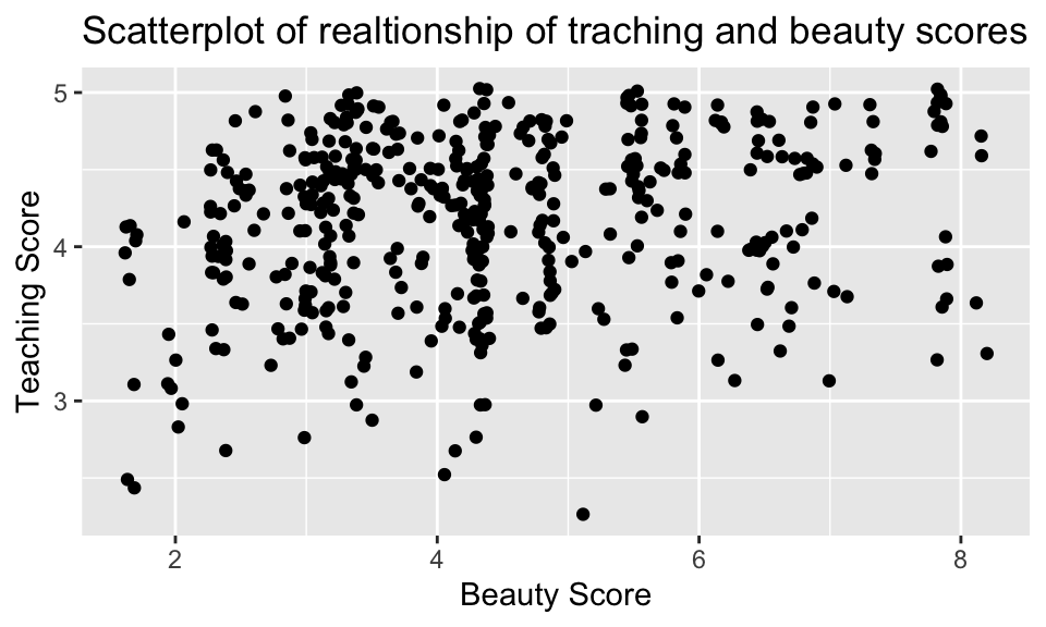
我們也可以使用 geom_smooth(method = "lm"),就能以最小平方法來適配模型,並畫出迴歸線(regression line),如:
evals_ch5 %>%
  ggplot(aes(x = bty_avg, y = score)) +
  geom_jitter() +
  geom_smooth(method = "lm", se = FALSE, formula = 'y ~ x') +
  labs(x = "Beauty Score",
       y = "Teaching Score",
       title = "Relationship between teaching and beauty scores")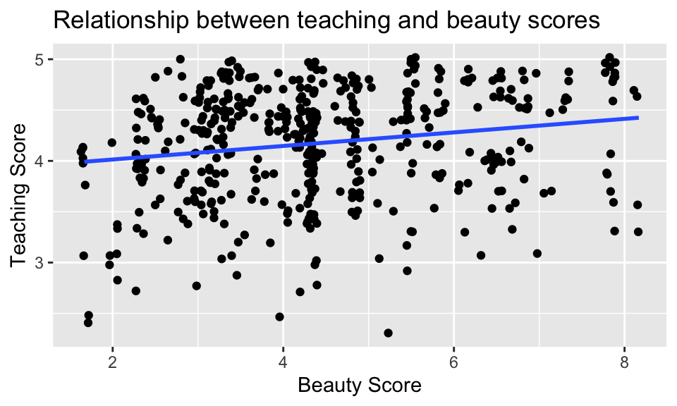
事實上,藍色線段的斜率恰等於上節所算出的相關係數 0.0187。不過,雖然相關係數與迴歸線的斜率的正負號通常相同,但其值通常不同。
23.1.2 簡單線性迴歸
如何進行簡單線性回歸?定義一迴歸線 \(\hat{y} = \hat{b}_0 + \hat{b}_1\cdot x\),我們可以:
使用
lm()函數適配迴歸模型,然後存在score_model中。把
score_model丟到套件moderndive中的get_regression_table()函數得到 regression table。
score_model <- lm(score ~ bty_avg, data = evals_ch5)
get_regression_table(score_model)
## # A tibble: 2 × 7
## term estimate std_error statistic p_value lower_ci upper_ci
## <chr> <dbl> <dbl> <dbl> <dbl> <dbl> <dbl>
## 1 intercept 3.88 0.076 51.0 0 3.73 4.03
## 2 bty_avg 0.067 0.016 4.09 0 0.035 0.099簡而言之,我們適配出的迴歸模型即
\[
\begin{aligned}
\hat{y} &= \hat{b}_0 +\hat{b}_1 \cdot x\\
\widehat{\rm score} &= 3.88 + 0.067 \cdot {\rm bty\_avg}
\end{aligned}
\]
這說明了,當 bty_avg 每增加 1 單位,score 平均會增加 0.067 單位。不過要注意的是,這是相關,而不是因果;即這是 associated increase,而非 causal increase。
23.1.3 Observed/fitted values and residuals
如果我們想看個別的點的預測值與殘差呢?我們可以 get_regression_points() 來完成這件事,如:
regression_points <- get_regression_points(score_model)
head(regression_points)
## # A tibble: 6 × 5
## ID score bty_avg score_hat residual
## <int> <dbl> <dbl> <dbl> <dbl>
## 1 1 4.7 5 4.21 0.486
## 2 2 4.1 5 4.21 -0.114
## 3 3 3.9 5 4.21 -0.314
## 4 4 4.8 5 4.21 0.586
## 5 5 4.6 3 4.08 0.52
## 6 6 4.3 3 4.08 0.2223.2 解釋變數為類別變數
世界上各國的預期壽命有什麼差異?各個大陸的人的預期壽命之間有何差異?同個大陸之間,預期壽命的分佈又是如何呢?
我們可以使用套件 gapminder 中的 gapminder 這個 data frame 來嘗試回答這個問題。其中,結果變數 \(y\) 是國家的預期壽命,一個連續變數;解釋變數 \(x\) 是國家屬於哪大洲,一個類別變數。資料詳情可以參照套件說明。
23.2.1 探索性資料分析
首先載入資料。我們觀察的焦點放在 2007 年的狀況,並且我們需要 country、lifeExp、continent 的資料。
library(gapminder)
gapminder2007 <- gapminder %>%
  filter(year == 2007) %>%
  select(continent, country, lifeExp)
23.2.1.1 EDA:觀察原始資料
glimpse(gapminder2007)## Rows: 142
## Columns: 3
## $ continent <fct> Asia, Europe, Africa, Africa, Americas, Oceania, Europe, Asi…
## $ country <fct> "Afghanistan", "Albania", "Algeria", "Angola", "Argentina", …
## $ lifeExp <dbl> 43.828, 76.423, 72.301, 42.731, 75.320, 81.235, 79.829, 75.6…gapminder2007 %>% sample_n(size = 5)## # A tibble: 5 × 3
## continent country lifeExp
## <fct> <fct> <dbl>
## 1 Africa Congo, Dem. Rep. 46.5
## 2 Asia Kuwait 77.6
## 3 Africa South Africa 49.3
## 4 Africa Zambia 42.4
## 5 Europe Sweden 80.923.2.1.2 EDA:簡單的敘述統計
gapminder2007 %>%
  select(lifeExp, continent) %>%
  skim()
── Data Summary ────────────────────────
Values
Name Piped data
Number of rows 142
Number of columns 2
_______________________
Column type frequency:
factor 1
numeric 1
________________________
Group variables None
── Variable type: factor ───────────────────────────────────────────────────────────────────
skim_variable n_missing complete_rate ordered n_unique top_counts
1 continent 0 1 FALSE 5 Afr: 52, Asi: 33, Eur: 30, Ame: 25
── Variable type: numeric ──────────────────────────────────────────────────────────────────
skim_variable n_missing complete_rate mean sd p0 p25 p50 p75 p100 hist
1 lifeExp 0 1 67.0 12.1 39.6 57.2 71.9 76.4 82.6 ▂▃▃▆▇23.2.2 線性迴歸
23.2.3 Observed/fitted values and residuals
參考文獻
可以發現 Ismay and Kim (2019) 的說法與 Wickham and Grolemund (2016) 不太相同。↩︎