Chapter 7 Real Systems
Real systems are characterized by friction, turbulence, unrestrained expansion, temperature gradients and mixing of dissimilar substances and are therefore irreversible. Molecular disorder increases and the total entropy is no longer constant but is constantly increasing.
7.1 Entropy generation in real systems
A few numerical examples will now be done to illustrate how entropy is generated in real systems.
7.1.1 Friction
In thermal fluid systems friction is generally between the fluid and the containing surface. Turbulence will cause friction between fluid molecules.
Example
In the heat pump of an refrigerator, saturated liquid freon from the
condenser flows through a thin capillary tube to the inlet of the
evaporator. Due to fluid friction the pressure drops and because of the
drop in pressure, the liquid boils and a two phase liquid results.
Because this is an adiabatic process, the enthalpy stays constant and
because a vapour has a higher enthalpy than a liquid, the temperature of
the resulting two phase mixture must be lower than the temperature of
the initial saturated liquid. (The liquid must “sacrifice” some of its
internal energy to provide the energy to form a vapor.) Calculate the
entropy before and after the capillary tube. Assume the freon at the
inlet is saturated R134 liquid at \(35^\circ C\) and the pressure
downstream is \(100kPa\)
Solution
For an adiabatic capillary tube:
\[h_{in}=100.9{kJ}/{kg}=h_{out}\]
From the pressure and enthalpy at the outlet the rest of the variables can be calculated: \(T=-26.4^\circ C\) and \(x=0.385\). The entropy increased from \(0.3714 kJ/kg\cdot K\) to \(0.4106kJ/kg\cdot K\)
It is clear that the entropy increased and that entropy has therefore been “created”. The cause of this increase is friction in the capillary tube.
7.1.2 Unrestrained expansion
When gas is expanded in a piston/cylinder arrangement, the molecules of the gas is restrained by the piston. The molecules collide with the moving piston, transferring their energy to the piston. In a reversible process no pressure gradient in the gas exists. If the rate of expansion is increased, a pressure gradient may develop and the pressure at the moving boundary may be lower. Then the amount of work performed by the system decreases. (\(\delta W = P \delta V\)) The faster the expansion takes place, the more unrestrained it becomes, the bigger the pressure gradient becomes and the lower the amount of work performed.
Example
Consider a balloon, containing \(1kg\) of air at \(100kPa\) and \(25^\circ C\)
bursting in an evacuated adiabatic container. The final pressure in the
container is \(10kPa\). Calculate the change in the entropy of the air.
Solution
Because the process is taking place in a vacuum, the pressure at the
boundary of the expanding gas is zero. No work is therefore performed.
Because no heat transfer takes place the internal energy stays constant.
For an ideal gas the internal energy is not dependent on pressure and
therefore the temperature of the gas does not change. The change in
entropy is therefore given by:
\[s_2-s_1=-R\ell n \frac {P_2}{P_1}=-0.287\ell n \frac{10}{100}=0.66\frac{kJ}{K}\]
It is clear the the entropy at the end of the process is more than at the beginning and because this is an adiabatic process, that entropy has been created.
If a balloon bursts in the earth’s atmosphere, the pressure at the boundary of the expanding gas is equal to the ambient pressure and some work is necessary to “push away” the atmosphere — therefore some work will be performed and the temperature of the gas will drop. However this is still not a reversible process and a pressure gradient will exist — causing the loud sound when a balloon bursts.
7.1.3 Heat transfer over a temperature difference
A temperature difference is necessary to provide the driving force for heat transfer. In reversible systems we assumed an infinitely small temperature difference leading to an infinitely slow rate of heat transfer. In real systems a finite temperature is necessary to make a finite rate of heat transfer possible.
Example
Consider a system consisting of two TERs. The one at 400K and the other
at 300K. 100kJ of heat is transferred between them. Calculate the change
in entropy of the system.
Solution
The heat will flow from the 400K TER to the 300K TER. The entropy of the
400K TER will decrease:
\[\Delta S_{400K}=\frac{-100}{400}=-0.25\frac{kJ}{K}\] The entropy of
the 300K TER will increase:
\[\Delta S_{300K}=\frac{100}{300}=0.3\dot3\frac{kJ}{K}\] The total
change is an increase of \(0.083\dot3 \thinspace kJ/K\)
In principle it is possible to install a heat engine between the two TERs above and generate work from the 100kJ of heat released by the high temperature TER. A reversible heat engine will generate no entropy. In the irreversible process above the ability of the high temperature heat to do work was destroyed and in the process, entropy was generated.
Heat can also flow at a certain rate across the boundary of a TER. \(\Delta \dot S\) is then rate at which the entropy of the TER is changing and it can therefore be seen as a “stream of entropy” that flows out of – or into the TER. The rate (or quantity) of entropy transfer across any boundary is dependent on the rate (or quantity) of heat as well as the temperature of the heat as can be seen from the definition of entropy:
\[dS=\frac{\delta Q}{T}\]
7.2 Entropy in real systems
In order to determine where entropy is generated in the system, the “flow” and generation of entropy in the system must be studied:
As all the energy in boundary and shaft work as well as kinetic and potential energy is available to perform work, they are free of entropy. As stated before: There is no entropy transfer associated with the transfer of energy as work or power.
Entropy is also a property. Therefore the rate of entropy transfer associated with mass transfer in an open system is equal to \(\dot m s [\frac{kJ}{K \cdot s}]\). The entropy associated with the mass in a closed system is equal to \(ms [\frac{kJ}{K}]\).
Entropy transfer is also associated with heat transfer. The entropy transferred with heat is determined by the temperature of the heat where it crosses the system boundary.
In any real process, entropy is generated (\(\dot S_{gen}>0\)) in open systems and (\(S_{gen}>0\)) in closed systems . In a reversible process the total entropy stays constant (\(S_{gen}=0\) or \(\dot S_{gen}=0\))
7.2.1 Internally reversible systems
By locating all irreversibilities outside the system boundary, an internally reversible system results. The principles of reversible processes (\(S_{gen}=0\) or \(S_{total}=Constant\)) can now be applied on the system by using the concept of entropy transfer. This sometimes make it possible to solve problems that could not be solved otherwise.
Example
One kilogram steam in a piston cylinder arrangement at \(300kPa\) and
\(200^\circ C\) is compressed at constant temperature to a pressure of
\(400kPa\), releasing heat to the environment at \(25^\circ C\). Calculate
the work required analytically as well as the entropy generated.
Solution
Because there is not a simple relationship between the pressure, volume
and temperature for steam, work has previously been determined
numerically (Paragraph
3.2.2). However, the First Law contains a work
term and can be used if the amount of heat exchanged can be determined.
The heat exchange takes place over the temperature difference between
the steam and the environment and this is an irreversible process and
entropy is generated. The entropy generated can only be calculated if
the amount of heat transferred is known – and that is what we want to
determine! So we are stuck. But by defining the steam as the system, an
internally reversible process results and the entropy transfer across
the system boundary can be calculated because the temperature of the
boundary is uniform and constant. The irreversibility is located outside
the system and does not influence the calculations. An entropy “balance”
can be done for the steam. The change in entropy of the steam is equal
to the transfer of entropy because it is an (internally) reversible
process.
\[m(s_1-s_2)=\frac{Q_{out}}{T_{system \thinspace boundary}}\]
The heat released can now be calculated: \[Q_{out}=T_{boundary}\times m(s_1-s_2)= (200+273.15)(7.3115-7.1706)=66.67kJ\]
From the First Law: \[W_{in}=m(u_2-u_1)+Q_{out}=(2646.83-2650.65)+66.67=62.86kJ\]
This means work was required to compress the steam, which makes sense. Note that the internal energy changed due to the change in pressure because steam is not an ideal gas. For an ideal gas the heat exchange would have been equal to the work.
The entropy generated with the transfer of heat through the wall of the cylinder, across the temperature difference, can now be calculated. The system boundary is now the outside of the wall of the cylinder which is at ambient temperature. \(S_{gen}\) is always bigger than zero. It is as if entropy has been added to the system. An entropy balance becomes:
\[ms_1+S_{gen}=ms_2+\frac{Q_{out}}{T_{ambient}}\]
The amount of entropy generated is \(0.0827\frac{kJ}{K}\)
7.2.2 Internally irreversible systems
Because entropy generation impacts negatively on the efficiency of energy conversion into work, it may be necessary to include the irreversibility in the system to quantify its efficiency. In the case of real turbines and compressors irreversibility is necessarily part of the system and must be taken into consideration. The efficiency of internally irreversible systems are often determined by comparing their real performance to the performance of a reversible system as in the figure below:
7.2.2.1 Turbines
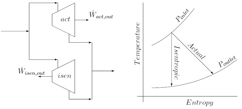
The isentropic efficiency is given by the actual power delivered by a turbine, divided by the power a isentropic turbine, with the same inlet conditions \((\dot m ;P_{in} ; T_{in})\) and the same outlet pressure \((P_{out})\), would have delivered:
\[\eta_{turbine}=\frac{\dot W_{actual}}{\dot W_{isentropic}}\]
Although they have the same outlet pressure56, the outlet temperature of the actual turbine will be higher than that of the isentropic turbine because the enthalpy in the inlet gas is not converted as efficiently into power due to irreversibilities such as friction and turbulence of the fluid passing through the actual turbine.
Example
Suppose the Helium turbine on page is not isentropic but has an
isentropic efficiency of 90% Calculate the power delivery and outlet
temperature of the actual turbine.
Solution
The isentropic power the turbine delivers is \(2782.5kW\). The actual
power is therefore:
\[\dot W_{actual}=0.9\times 2782.5=2504.2kW\]
As a smaller fraction of the energy in the steam has been converted into power, the outlet temperature of actual turbine will be higher than that of the isentropic turbine. An energy balance for the actual turbine:
\[\dot W_{actual} = \dot m C_{p}(T_{in}-T_{out,actual})\]
gives a value of \(632.0\)K for \(T_{out,actual}\) which is higher than the isentropic outlet temperature of \(605.2\)K
7.2.2.2 Compressors
The power required by an isentropic compressor will be lower than the power required by a real compressor because of turbulence and friction in the real compressor. Therefore the efficiency for compressors is given by:
\[\eta_{compressor}=\frac{\dot W_{isentropic}}{\dot W_{actual}}\]
Example
Saturated steam at \(100kPa\) flows at a rate of \(1kg/s\) to a compressor.
The pressure at the outlet is \(200kPa\) and the temperature
\(180^\circ C\). Calculate the isentropic efficiency of the compressor.
Solution
The efficiency is given by:
\(\eta_{compressor}=\frac{\dot W_{isentropic}}{\dot W_{actual}}\) The
actual power required is given by an enthalpy balance:
\[\dot m h_{in}+W_{actual}=\dot m h_{out,actual}\]
The actual outlet conditions is given in the problem statement. Interpolation give the enthalpy at he outlet: \(2829.8\frac{kJ}{kg}\) and the actual power required is calculated from an energy balance:
\[\dot W_{actual}=2829.8-2675.1=154.5kW\]
The isentropic power required, is given by an enthalpy balance over an isentropic compressor with the same inlet conditions and outlet pressure as the actual compressor. (Just as the outlet temperatures of a real and isentropic turbine will be different as shown in the T-s diagram above, the outlet temperatures of the real and isentropic compressors will be different.)
\[\dot m h_{in}+W_{isentropic}=\dot m h_{out,isentropic}\]
The value of the outlet pressure is known and the outlet entropy is the same as the inlet entropy. These two values can be used to determine the (isentropic) outlet enthalpy. At \(200kPa\) and an entropy of \(7.3593kJ/kg\cdot K\) the enthalpy is \(2803kJ/kg\). This gives the isentropic power required: \(128kW\) and an isentropic efficiency of \(\eta=\frac{128}{154}=83\%\).
It is left to the reader to verify that the outlet temperature of the isentropic compressor is \(166.8^\circ C\)
7.3 The significance of entropy generation
In the previous chapter entropy was considered from a statistical viewpoint. (Entropy is a measure of molecular disorder.) Entropy can also be described as: An indication of the unavailability of heat, internal energy and enthalpy to perform work. It is clear from the examples in Paragraph 7.1 that the generation of entropy is associated with a reduced work output.
Example
Consider two piston cylinder arrangements containing \(1kg\) of Helium at
\(25^\circ C\) The Helium in the first cylinder is at atmospheric pressure
(\(85kPa\)) and the other at \(170kPa\). Calculate the difference in entropy
between the two. Calculate the work performed if both of them are
expanded isentropically to the ambient pressure of \(85kPa\)
Solution
As the temperatures are the same, the difference in entropy is given by:
\[s_{85kPa}-s_{170kPa}=-0.287\ell n \frac{85}{170}=0.199\frac{kJ}{kg \cdot K}\]
The entropy of the Helium at \(170kPa\) is the lower of the two. The Helium at ambient pressure cannot do any work. For the calculation of work done in the expansion of the Helium at \(170kPa\), the First Law can be used. But first the temperature after expansion to \(85kPa\) has taken place has to be calculated:
\[{T_2}={T_1} \left(\frac{P_2}{P_1}\right)^\frac{k-1}{k}=298.15\left(\frac{85}{170}\right)^\frac{1.667-1}{1.667}=225.9K\]
The First Law for an adiabatic system:
\[W_{out}=m\times C_v (T_1-T_2)=3.116(298.15-225.9)=225kJ\]
Even though the internal energies are the same, the Helium at the higher pressure can perform more work than the Helium at the lower pressure. Also the Helium at the higher pressure has the lower entropy. This illustrates the fact the entropy is an indication of the unavailability of internal energy to do work.
This has implications for the efficiency of converting internal energy, enthalpy and heat into work. As entropy is generated in real systems, the ability of the internal energy, enthalpy and heat to perform work, will decrease. The generation of entropy should therefore be minimized if work output is to be maximized. It can be shown (Sonntag and Borgnakke 2012 Par. 10.1) that the difference between the power produced/consumed by an actual and a reversible adiabatic device operating between the same inlet and outlet conditions \(\mid \dot W_{actual} - \dot W_{reversible} \mid = T_0 \dot S_{gen}\) where \(T_0\) is the ambient temperature in Kelvin.57 The equation can therefore be used to calculate the difference between the power consumption of a reversible and real compressor or the difference in the power produced by real and reversible turbine or the reversible power that could have been produced by a condenser – had all the processes been reversible. The derivation of this equation is beyond the present scope of this notes.
The constant pressure curve in the \(T-s\) graph have a specific shape. From the equations in Paragraph 6.3.2 it is clear that for a perfect gas, the relationship between entropy and temperature at a specific (constant) pressure, is logarithmic. For ideal gas air, the entropy at \(100kPa\) as function of temperature can be read directly form the Ideal Gas Air tables. For steam, consult Borgnakke (Sonntag and Borgnakke 2012 Figure 6.7)↩︎
Note that the outlet conditions of an isentropic turbine as on page differs from the outlet conditions of the real turbine. This equation is therefore not applicable when real and isentropic devices are compared↩︎