Chapter 7 Chapter 7: Getting Started with Generalized Linear Models

Response variables in linear model-based analyses have several common features including that:
- We assume they are continuous variables that can take negative and positive values and can be fractins
- We also assume that these data are bounded (but in practice, sometimes they are not)
- The models assume normally distributed residuals
- The model also assumes a constant mean-variance relationship
Often there are response variables in which the normality assumption is violated
Examples of data that violate assumptions:
- Integer valued data that is bounded and cannot be fractioned or negative (i.e. the number of people)
- Binary data (i.e. presence/absence data)
Historically for these types of data, transformations are employed such as log10 transformations for counts or arcsin(sqrt()) transformations for proportion data
This is where the generalized linear model (GLM) may be utilized

7.0.1 Counts and Proportions and the GLM

Count data:
- Are bounded by 0 and infinity
- Violate the normality assumption
- Do not have a constant mean-variance relationship
Example:
- How the number of offspring a female may produce over her lifetime relates to body size
  - How a rate of occurence of events (births) depends on other variables (body size)
Proportion data - data are often binary
- flowering data
- animal death
- species sex ratios
These occurences are often related to 1+ explanatory variables
These data are binomial

7.0.2 Key terms of GLM models

Family
- The probability distribution that is assumed to describe the response variable
- In other words, it’s a mathematical statement of how likely events are
- Poisson and binomial distributions are examples of families
Linear predictor
- This is an equation that describes how the different predictor variables (explanatory variables) affect the expected value of the response variable
Link function
- Describes the mathematical relationship between the expected value of the response variable and the linear predictor, linking, the two aspects of the GLM
glm() will be used to create generalized linear models

7.1 Counts and rates - Poisson GLMs

7.1.1 Counting Sheep - the data and question

In this dataset, the response variable is a count variable
We aim to understand how the rate of occurence of events depends on 1 or more explanatory variables
Dataset backstory:
- It’s about a specific population of sheep
- These sheep are on an island off the west coast of Scotland
- They are unmanaged/feral population of Soay sheep
- There has been a lot of scientific interest on this population to study how the population is evolving
- Several studies have been done on female (ewe) fitness
  - One way to measure fitness is to count the total number of offspring born to a female during her life - ‘lifetime reproductive success’
    - response variable = counts of offspring, which are poorly approximated by a normal distribution
question: Does lifetime reproductive success increase with ewe bodymass?
- Do larger ewes produce more offspring?
- If so, then is there a heritable difference in body mass - is there selection pressure on this trait?

install.packages("ggplot2",  repos = "https://cran.us.r-project.org")
install.packages("dplyr",  repos = "https://cran.us.r-project.org")
install.packages("ggfortify",  repos = "https://cran.us.r-project.org")

library(ggplot2)
library(dplyr)
library(ggfortify)

soay <- read.csv("/Users/peteapicella/Documents/R_tutorials/GSwR/SoaySheepFitness.csv", header = TRUE) 
str(soay)

## 'data.frame':    50 obs. of  2 variables:
##  $ fitness  : int  4 3 2 14 5 2 2 5 8 4 ...
##  $ body.size: num  6.37 7.18 6.16 8.6 7.33 ...

Visualize the data:

ggplot(soay, aes(x = body.size, y = fitness)) + 
  geom_point() + 
  geom_smooth(method = "lm", se = FALSE) + #applies linear regression (blue) line 
  geom_smooth(span = 1,                    #determines how wiggly the curve is 
              colour = "red", se = FALSE) + #applies a non-linear and more  flexible statistical model  
  xlab("Body mass (kg)") + ylab("Lifetime fitness")

## `geom_smooth()` using formula 'y ~ x'

## `geom_smooth()` using method = 'loess' and formula 'y ~ x'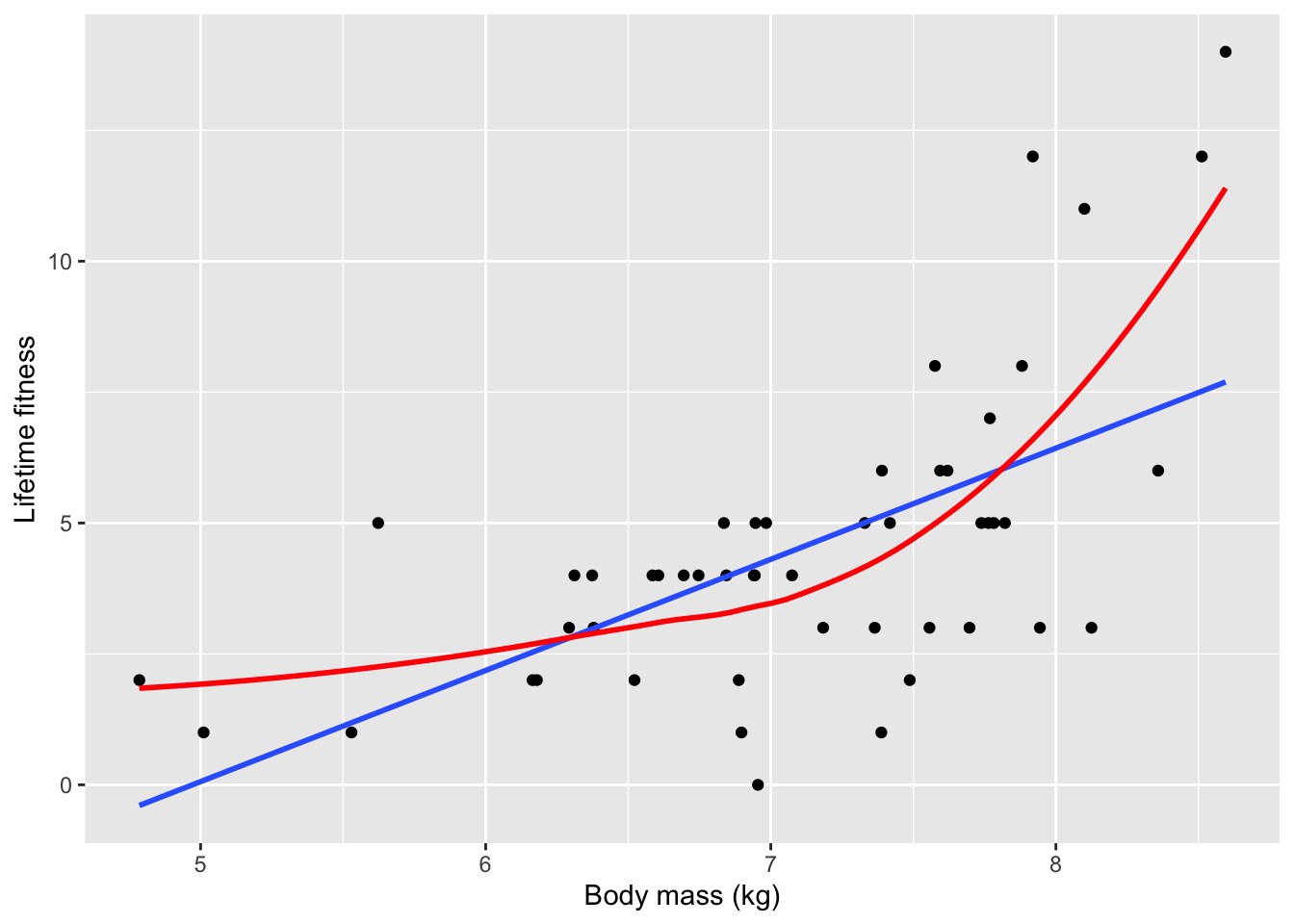

Based on the loose fitting models, there is a strong positive relationship between fitness and body size in which larger ewes have more offspring over time
- Larger ewes have more resources to allocate to reproduction
The red line clearly captures the relationship more effectively than the blue one
The upward trending of the red line is an issue of non-linearity
There are also subtler issues with the data
To really understand these problems, the authors want to analyze the data the incorrect way and then right the wrongs with the correct analysis after

7.2 Doing it wrong

Create an inappropriate model using the linear model approach:

soay.mod <- lm(fitness ~ body.size, data = soay)
autoplot(soay.mod, smooth.colour = NA)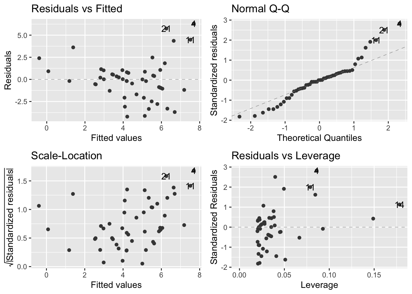

Almost all of our assumptions are violated

7.2.1 Doing it wrong: diagnosing the problems

Residuals vs fitted values (upper left):
- Suggests that the systematic part of the model is inappropriate because there is a pattern of the datapoints
  - In fact, the U-shape of the data indicate that the straight-line model fails to account for the curvature in the relationship between our two variables
- Fitness is underestimated at small body sizes
- Fitness is overestimated at larger body sizes
Normal Q-Q plot (upper right):
- Most of the points should be on the dashed diagnonal line and they are not
  - Many of the points in positive territory are above the line
  - Many of the points in negative territory are below the line
- We see this pattern because the distribution of residuals is not symmetrical
  - In this case, it is skewed to the right

Visualize rightward skew through a histogram:

ggplot(soay, aes(x=body.size))+ geom_histogram(bins=20)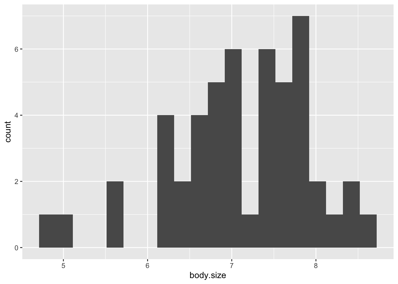

Scale location plot (bottom left):
- There is a clear pattern that shows a positive relationship between the absolute size of the residuals and the fitted values
  - This reflects the way the fitness values are scattered around the red line: there is more vertical spread in the data at larger fitness values
  - Based on this, we can say that there is a positive mean-variance relationship in the data
  - In other words, large predicted fitness values are associated with more variation in the residuals
  - This is typical of count data
Residuals-leverage plot (bottom right):
- This plot is not too bad
- There are no extreme standardized residual values
  - No obvious outliers
- None of the observations are having an outsized effect on the model

Overall, the normal linear regression is not doing a good job of describing the data

7.2.2 The Poisson distribution - a solution

The normality assumption built into the linear regression model is not appropriate for these data - Properties of a normal distribution:
- Concerns continuous variables (can assume fractional values)
  - Count data are discete (i.e. a ewe can produce 0,1,2, etc. lambs)
- Normal distribution allows for negative values
  - Count data must be positive (i.e. ewe cannot have -2 offspring)
- Symmetry.
  - Count data often are asymmetrical
Poisson distribution is a good starting point for the analysis of certain forms of count data

A visual for understanding the Poisson distribution:

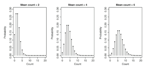
The above figure displays three Poisson distributions and each has a different mean
The x-axis has a range of different possible values and the y axis has the probability of each value
Reasons why the poisson distribution is a good model for the Soay data:
- Only discete counts are possible
- Data are bounded at 0
- Very large counts are possible and in the scope of the model; however, their occurence is unlikely
- Variance of the distribution increases as the mean of distribution is increased
  - This corresponds to the widening of the base the distribution with a higher mean
The poisson distribution is best equipped for unbounded count data
- What unbounded here refers to is just that there is no uppper limit to the values that the count variable may take
- There are obvious biological constraints, but we don’t actually know the limit

7.3 Doing it right - the Poisson GLM

7.3.1 Anatomy of a GLM

GLM is comprised of three key terms: family, linear predictor, the link function
family:
- This is the error aspect of the GLM
- Determines what kind of distribution is used to describe the response variable. Options:
  - Poisson distribution
  - Binomial distribution
  - Gamma distribution (positive valued, continuous variables)
  - Other exotic versions
- Each option is appropriate for specific types of data
linear predictor:
- Every time a model is built with the lm() function, some data and an R formula must be supplied to define the model
- The R formula defines the linear predictor
- Soay example:
  - inappropriate regression with model: lm(fitness ~ body.size, data = soay)
  - This tells R to build a model for the predicted fitness given an intercept and body size slope term: Predicted fitness = Intercept + Slope x Body size
  - The linear predictor is ‘Intercept + Slope x Body size’
    - so it’s basically just the model
  - Coefficients shown by summary(soay.mod) are just the intercepts and slopes of th linear predictor
The link function:
- A model that cannot make impossible predictions is preferred
  - You can plug numbers into the formul that will produce illogical outputs such that:
    - A negative number of offspring in this sheep example
  - With the GLM, instead of trying to model the predicted values of the response variable directly, we model a mathematical transformation of the prediction
    - The transformation is the link function
- Using a Poisson GLM to model the fitness vs body mass relationship, the model for the predicted fitness would look like this:
  - Log[Predicted fitness] = Intercept + Slope x Body size
    - This is a natural log in this case
    - The link function in a standard Poisson GLM is always natural log
- Instead of the linear predictor describing fitness directly, it relates the natural logarithm of predicted fitness to body size
  - This must be positive, but the log transformed value can take any value
- Solve for predicted fitness to get:
- Predicted fitness = e^{Intercept + Slope x Body size}
A Poisson GLM for the Soays sheep implies an exponential relationship between fitness and body mass
- linear model does not mean a linear relationship
The link function allows for the estimation of the paramenteres of a linear predictor that is apporpriate for the data
- This is accomplished by transforming the response ‘scale’ to the scale of the linear predictor, which in this case a natural log scale, which is defined by the link function
- This is can be visualized in the following figure:

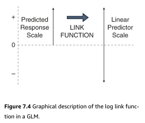
Figure:
- Count data is bounded by 0 and positive infinity
  - Predicted values must be greater than 0 to be valid for count data
- But, to do effective statistics, we need to operate on a scale that is unbounded
- Using the link function accomplishes this
- It moves us from the positive numbers (predicted average counts) scale to the whole number line (the linear predictor) scale

7.3.2 Doing it right - actually fitting the model

Build the GLM:

soay.glm <- glm(fitness ~ body.size, data = soay, 
                family = poisson(
                  link = log)) #this line is unnecessary because the log link function is the default for poisson glm

7.3.3 Doing it right - the diagnostics

autoplot(soay.glm, smooth.colour = NA)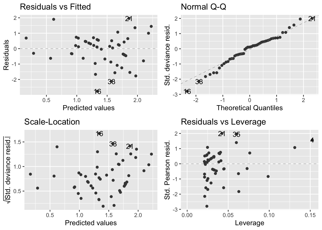

Overall, the diagnostics look much better
- Residuals vs fitted values (upper left):
  - The systematic aspect of the model is fairly appropriate
    - There is no clear pattern in the relationship apart from a very slight upward trend
    - Not enough to be concerned with though
- Normal Q-Q plot (upper right):
  - There is some departure from the dashed diagnonal line, but a perfect plot is not expected
  - Confirms that the distributional assumptions are okay
- Scale location plot (bottom left):
  - There is a slight positve relationship between the size of the residuals and the fitted values, but not too much of a concern
- Residuals-leverage plot (bottom right):
  - Shows no evidence that there are outliers or points having an outsized effect on the model
Keep in mind that when R does diagnostics for a GLM, it uses standardized deviance residuals
- This is a transformed version of raw residuals that make transformed residuals normally distributed if the GLM family that is being used is appropriate
- This means that if the chosen family is appropriate for the data, then the diagnostics should show that the residuals are normally distributed
- And the diagnostic plots can be evaluated in the same way as for a linear model because the tests are doing all the same jobs

7.3.4 Doing it right - `anova()` and `summary()`

Thus far it looks that fitnesss is positively related to body mass
The next step is to test hypotheses

Create Analysis of Deviance table for the GLM:

anova(soay.glm)

## Analysis of Deviance Table
## 
## Model: poisson, link: log
## 
## Response: fitness
## 
## Terms added sequentially (first to last)
## 
## 
##           Df Deviance Resid. Df Resid. Dev
## NULL                         49     85.081
## body.size  1   37.041        48     48.040

“Deviance” here is closely related to the idea of likelihood, which is a general tool for doing statistics
- Short explanation of likelihood: provides us with a measure of how probable the data would be if they had really been produced by that model
  - Using likelihood, you can find a set of best-fitting model coefficients by picking values that maximize likelihood
  - Also, sum of squares and mean squares allow for the comparison of different models when normality is assumed
  - Likelihood (and deviance) do the same thing for GLMs
no p values in this table
- Total deviance for NULL (fitness) is 85.081 and body.size explains 37.041 units of the deviance - So bodysize accounts for almost half of the deviance. This is very large.
- There is no p value because R wants the type of test to calculate it to be specified
p values in the GLM involve a \(\chi\)\(^{2}\) distribution rather than an F-distribution (this does not mean that a \(\chi\)\(^{2}\) test is to be performed)

Specifiy the type of test:

anova(soay.glm, test = "Chisq")

## Analysis of Deviance Table
## 
## Model: poisson, link: log
## 
## Response: fitness
## 
## Terms added sequentially (first to last)
## 
## 
##           Df Deviance Resid. Df Resid. Dev  Pr(>Chi)    
## NULL                         49     85.081              
## body.size  1   37.041        48     48.040 1.157e-09 ***
## ---
## Signif. codes:  0 '***' 0.001 '**' 0.01 '*' 0.05 '.' 0.1 ' ' 1

The test statistic has a value of 37.041
- The corresponding p value is very small
- This is unsurprising given the strong relationship visualized in the scatterplot
- This is a likelihood ratio test
This means that fitness does vary positively with body size and there is selection pressure on higher body mass

Find out more about the model:

summary(soay.glm)

## 
## Call:
## glm(formula = fitness ~ body.size, family = poisson(link = log), 
##     data = soay)
## 
## Deviance Residuals: 
##     Min       1Q   Median       3Q      Max  
## -2.7634  -0.6275   0.1142   0.5370   1.9578  
## 
## Coefficients:
##             Estimate Std. Error z value Pr(>|z|)    
## (Intercept) -2.42203    0.69432  -3.488 0.000486 ***
## body.size    0.54087    0.09316   5.806 6.41e-09 ***
## ---
## Signif. codes:  0 '***' 0.001 '**' 0.01 '*' 0.05 '.' 0.1 ' ' 1
## 
## (Dispersion parameter for poisson family taken to be 1)
## 
##     Null deviance: 85.081  on 49  degrees of freedom
## Residual deviance: 48.040  on 48  degrees of freedom
## AIC: 210.85
## 
## Number of Fisher Scoring iterations: 4

Table output:
- First chunk is self explanatory
- Second chunk - “useless” summary of specially scaled (deviance) residuals
- Third chunk - coefficients
  - model is a line so there are only two coefficients - the intercept and a slope
  - Each coefficient has a standard error to tell us how precise it is and a z-value to help us determine if the estimate is significantly different from 0 and the associated p value
- Fourth chunk - dispersion parameter - more on this later
- Fifth chunk - summaries of the null deviance, residual deviance, and their dfs
  - null deviance - measure of all the ‘variation’ in the data
  - residual deviance - measure of what is left over after fitting the model
    - The bigger the difference in these two values, the more variation is explained by the model
- AIC = Akaike information criterion (not analyzed in this text)
- Number of Fisher Scoring iterations - not important
Upon looking at the original scatterplot that helped visualize the data and this summary table, it might be confusing to see that the intercept has a negative value
- But remember that the link function is being used to predict the natural logarithm of lifetime fitness, not actual fitness
We will revisit the overdispersion concept later in the chapter

7.3.5 Making a beautiful graph

Need to generate a set of new x values

Generate new x values:

min.size = min(soay$body.size)
max.size = max(soay$body.size)

new.x = expand.grid(body.size = 
                      seq(min.size, max.size, #the new x values will be between these two parameters 
                          length = 1000)) #R generates 1000 values between

Now the predict() function can be used:
- predict() is given three arguments: the GLM model, a value for newdata, and a request for standard errors
- Side note: predict() for glm does not have a confidence interval argument, so they have to be manually rendered into the dataframe

new.y <- predict(soay.glm, 
                 newdata = new.x, #instructs R to use the new x values 
                 se.fit = TRUE) #provides standard errors.predict() for glm() doesn't have an interval = confidence argument
new.y = data.frame(new.y) #converts new.y into a dataframe 
head(new.y)

##         fit    se.fit residual.scale
## 1 0.1661991 0.2541777              1
## 2 0.1682619 0.2538348              1
## 3 0.1703247 0.2534919              1
## 4 0.1723874 0.2531491              1
## 5 0.1744502 0.2528063              1
## 6 0.1765130 0.2524635              1

Combine new x values with new y values:

addThese = data.frame(new.x, new.y)
names(addThese)[names(addThese) == 'fit'] <- 'fitness' #this will match the original data 

head(addThese)

##   body.size   fitness    se.fit residual.scale
## 1  4.785300 0.1661991 0.2541777              1
## 2  4.789114 0.1682619 0.2538348              1
## 3  4.792928 0.1703247 0.2534919              1
## 4  4.796741 0.1723874 0.2531491              1
## 5  4.800555 0.1744502 0.2528063              1
## 6  4.804369 0.1765130 0.2524635              1

Calculate and include the confidence intervals in the dataframe:

addThese = mutate(addThese, 
                  lwr = fitness -1.96 * se.fit, #this and the line below add the lower and upper bounds of the 95% CI 
                  upr = fitness +1.96 * se.fit)
head(addThese)

##   body.size   fitness    se.fit residual.scale        lwr       upr
## 1  4.785300 0.1661991 0.2541777              1 -0.3319891 0.6643874
## 2  4.789114 0.1682619 0.2538348              1 -0.3292543 0.6657781
## 3  4.792928 0.1703247 0.2534919              1 -0.3265195 0.6671689
## 4  4.796741 0.1723874 0.2531491              1 -0.3237848 0.6685597
## 5  4.800555 0.1744502 0.2528063              1 -0.3210501 0.6699506
## 6  4.804369 0.1765130 0.2524635              1 -0.3183156 0.6713415

Visualize the data with our new model + predicted values:

ggplot(soay, aes(x = body.size, y = fitness)) + 
  geom_point(size = 3, alpha = 0.5) + 
  geom_smooth(data = addThese, 
              aes(ymin = lwr, ymax = upr), stat = 'identity') + 
  theme_bw()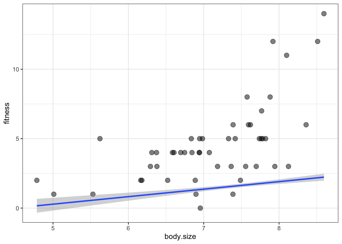

it didn’t work:

What happened is that the default scale for predict() is just the scale of the link function
The link function uses a logarithmic scale
- This means that the predictions are the log of the expected fitness, but we want to plot the actual fitness values
To fix this, the inverse log must be applied to any y-axis variables in addThese
- To inverse log, we just have to exponentiate them

Recreate the y values:

min.size = min(soay$body.size)
max.size = max(soay$body.size)

new.x = expand.grid(body.size = seq(min.size, max.size, length = 1000)) 

new.y <- predict(soay.glm, 
                 newdata = new.x, 
                 se.fit = TRUE)  
new.y = data.frame(new.y) 
addThese = data.frame(new.x, new.y)
head(addThese)

##   body.size       fit    se.fit residual.scale
## 1  4.785300 0.1661991 0.2541777              1
## 2  4.789114 0.1682619 0.2538348              1
## 3  4.792928 0.1703247 0.2534919              1
## 4  4.796741 0.1723874 0.2531491              1
## 5  4.800555 0.1744502 0.2528063              1
## 6  4.804369 0.1765130 0.2524635              1

Exponentiate the y values:

addThese = mutate(addThese, 
                  fitness = exp(fit),
                  lwr = exp(fit - 1.96 *se.fit), 
                  upr = exp(fit - 1.96*se.fit)) 
head(addThese)

##   body.size       fit    se.fit residual.scale  fitness       lwr       upr
## 1  4.785300 0.1661991 0.2541777              1 1.180808 0.7174951 0.7174951
## 2  4.789114 0.1682619 0.2538348              1 1.183246 0.7194600 0.7194600
## 3  4.792928 0.1703247 0.2534919              1 1.185690 0.7214303 0.7214303
## 4  4.796741 0.1723874 0.2531491              1 1.188138 0.7234059 0.7234059
## 5  4.800555 0.1744502 0.2528063              1 1.190591 0.7253869 0.7253869
## 6  4.804369 0.1765130 0.2524635              1 1.193050 0.7273732 0.7273732

Revisulize the data:

ggplot(soay, aes(x = body.size, y = fitness)) + 
  geom_point(size = 3, alpha = 0.5) + 
  geom_smooth(data = addThese, 
              aes(ymin = lwr, ymax = upr), stat = 'identity') + 
  theme_bw()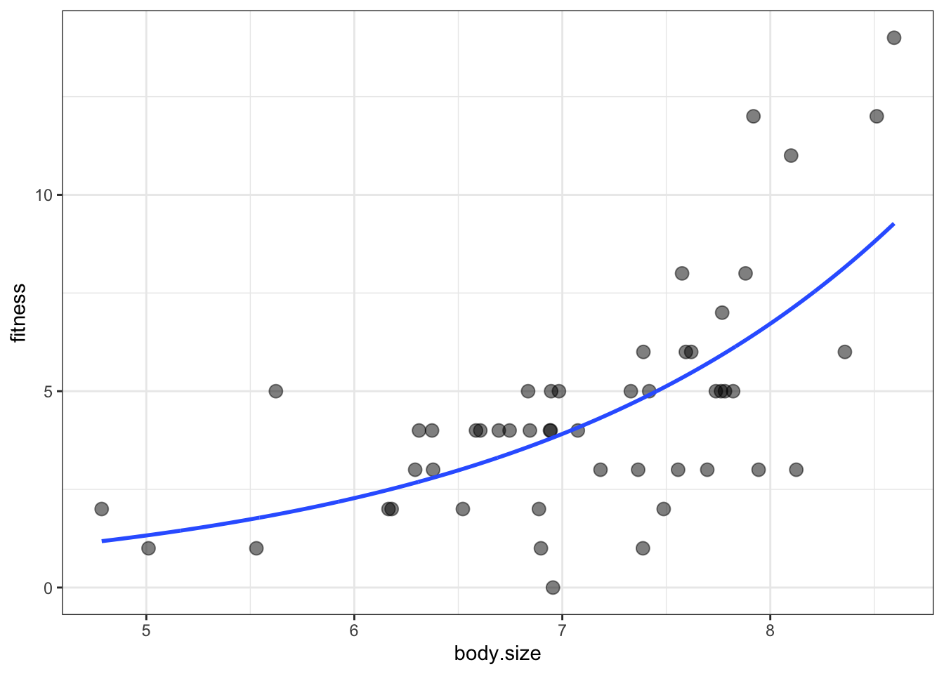

7.4 When a Poisson GLM isn’t good for counts

The previous data set was the best case scenario for a GLM and the simplest use case
Now we will work with more realistic data

7.4.1 Overdispersion

Overdispersion means ‘extra variation’
GLMs make strong assumptions about the nature of variability in the data
- We have seen how the variance increases with the mean
- For a Poisson distribution, the variance is equal to the mean
  - This assumption can only be true if you can account for every source of variation in the data (big assumption esp in biology)
- But Biology creates variation that cannot be measured or accounted for
- This is the source of the overdisperson problem
  - From non-independence in the data
    - Non-independence refers to the idea that some elements in the data are more similiar to one another than they are to other things
    - i.e. cannabis plants in experiment are more similiar to each other than a random plant
overdispersion sounds like BS but it can really mess up statistical output if it is ignored (i.e. p-values) and end up with false positives
What to do about it?
- First: detect it.

summary(soay.glm)

## 
## Call:
## glm(formula = fitness ~ body.size, family = poisson(link = log), 
##     data = soay)
## 
## Deviance Residuals: 
##     Min       1Q   Median       3Q      Max  
## -2.7634  -0.6275   0.1142   0.5370   1.9578  
## 
## Coefficients:
##             Estimate Std. Error z value Pr(>|z|)    
## (Intercept) -2.42203    0.69432  -3.488 0.000486 ***
## body.size    0.54087    0.09316   5.806 6.41e-09 ***
## ---
## Signif. codes:  0 '***' 0.001 '**' 0.01 '*' 0.05 '.' 0.1 ' ' 1
## 
## (Dispersion parameter for poisson family taken to be 1)
## 
##     Null deviance: 85.081  on 49  degrees of freedom
## Residual deviance: 48.040  on 48  degrees of freedom
## AIC: 210.85
## 
## Number of Fisher Scoring iterations: 4

If a GLM is working appropriately and there is no overdispersion, then residual deviance (48.040) and its degrees of freedom (48) should be equal
Perform \(\frac{residual~deviance}{residual~degrees~of~freedom}\)
Then the output is a ‘dispersion index (DI)’ which should be approximately 1
- If much bigger than 1, then the data are overdispersed
  - As a rule of thumb, if \(DI \ge 2\)
- If it is much less than 1, then the data are underdispersed (this is rare)
Fortunately, the soay data have normal dispersion levels
If data are overdispersed, then you can model the data differently
A simple fix is to change the family in glm() from family = poisson to family = quasipoisson
- a quasi model works just like the glm but it also estimates the dispersion index in a much more clever way than we did
- Once this index value is known, then R can adjust the p-values accordingly
Can also switch to a negative binomial family
- A negative binomial distribution is thought of as being more flexible than a Poisson distribution
- The variance increases with the mean, but in a less constrained way. The variance does not have to equal the mean

soay.glm2 <- glm(fitness ~ body.size, data = soay, 
                family = quasipoisson(
                  link = log)) 
summary(soay.glm2)

## 
## Call:
## glm(formula = fitness ~ body.size, family = quasipoisson(link = log), 
##     data = soay)
## 
## Deviance Residuals: 
##     Min       1Q   Median       3Q      Max  
## -2.7634  -0.6275   0.1142   0.5370   1.9578  
## 
## Coefficients:
##             Estimate Std. Error t value Pr(>|t|)    
## (Intercept) -2.42203    0.65967  -3.672 0.000605 ***
## body.size    0.54087    0.08851   6.111  1.7e-07 ***
## ---
## Signif. codes:  0 '***' 0.001 '**' 0.01 '*' 0.05 '.' 0.1 ' ' 1
## 
## (Dispersion parameter for quasipoisson family taken to be 0.9026887)
## 
##     Null deviance: 85.081  on 49  degrees of freedom
## Residual deviance: 48.040  on 48  degrees of freedom
## AIC: NA
## 
## Number of Fisher Scoring iterations: 4

The only difference between this summary statistics table and the original one for the soay glm is the p-values. They are based on a method that accounts for over/underdispersion
One more thing. Need to tell R to take into account the estimated dispersion by:

anova(soay.glm, 
      test = "F") #instead of Chisq

## Analysis of Deviance Table
## 
## Model: poisson, link: log
## 
## Response: fitness
## 
## Terms added sequentially (first to last)
## 
## 
##           Df Deviance Resid. Df Resid. Dev     F    Pr(>F)    
## NULL                         49     85.081                    
## body.size  1   37.041        48     48.040 37.04 1.157e-09 ***
## ---
## Signif. codes:  0 '***' 0.001 '**' 0.01 '*' 0.05 '.' 0.1 ' ' 1

7.4.1.1 Negative binomials

Use glm.nb() to build negative binomial models from the MASS package (base-R)
There is little else new that I need to learn
The default link function is the natural log, but can check ?glm.nb for alternatives
Neither quasi or negative binomial models appropriately deal with overdispersion that is caused by non-independence
- This is the job of mixed models, which will not be discussed in this text

7.4.2 Zero inflation

One specific source of overdispersion in Poisson-like count data is known as zero-inflation
This occurs when there are too many zeroes relative to the expected number for whichever distribution is being used
- If count is zero-inflated, you can often spot it with a chart of raw counts (i.e. spike at 0 on a bar chart - often results from zero-inflation)
Biological counts are often zero-inflated
- Occurs when binary results combine with a Poisson process

7.4.3 Transformations ain’t all bad

Sometimes transformations are appropriate, sometimes not
When in doubt, build the model and test the diagnostics
If the diagnostics look okay, then it’s probably fine to use the model
Advantages of using transformations:
- They work well when the data are far away from zero (no zeroes), but don’t span orders of magnitiude
- Can analyze “split-plot” designs fairly easily