Chapter 4 Chapter 4: Visualizing your data

4.1 The first step in every data analysis - making a picture

install.packages("ggplot2",  repos = "https://cran.us.r-project.org")
install.packages("dplyr",  repos = "https://cran.us.r-project.org")

library(ggplot2)
library(dplyr)

Read in the data

compensation <- read.csv("/Users/peteapicella/Documents/R_tutorials/GSwR/compensation.csv")

View dataframe & read the variables + the first few of their observations horizontally:

glimpse(compensation) #

## Rows: 40
## Columns: 3
## $ Root    <dbl> 6.225, 6.487, 4.919, 5.130, 5.417, 5.359, 7.614, 6.352, 4.975,…
## $ Fruit   <dbl> 59.77, 60.98, 14.73, 19.28, 34.25, 35.53, 87.73, 63.21, 24.25,…
## $ Grazing <chr> "Ungrazed", "Ungrazed", "Ungrazed", "Ungrazed", "Ungrazed", "U…

4.2 ggplot2: a grammar for graphics

Create base plot:

base_plot <-ggplot(compensation, aes(x = Root, y = Fruit, 
                                colour=Grazing)) + #colour: for the two levels of the categorical variable, Grazing
  geom_point()                                       
base_plot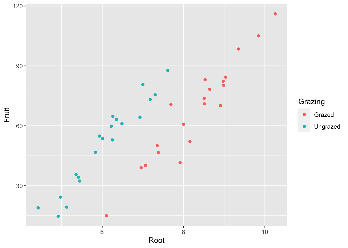

Render background white instead of gray:

base_plot + theme_bw()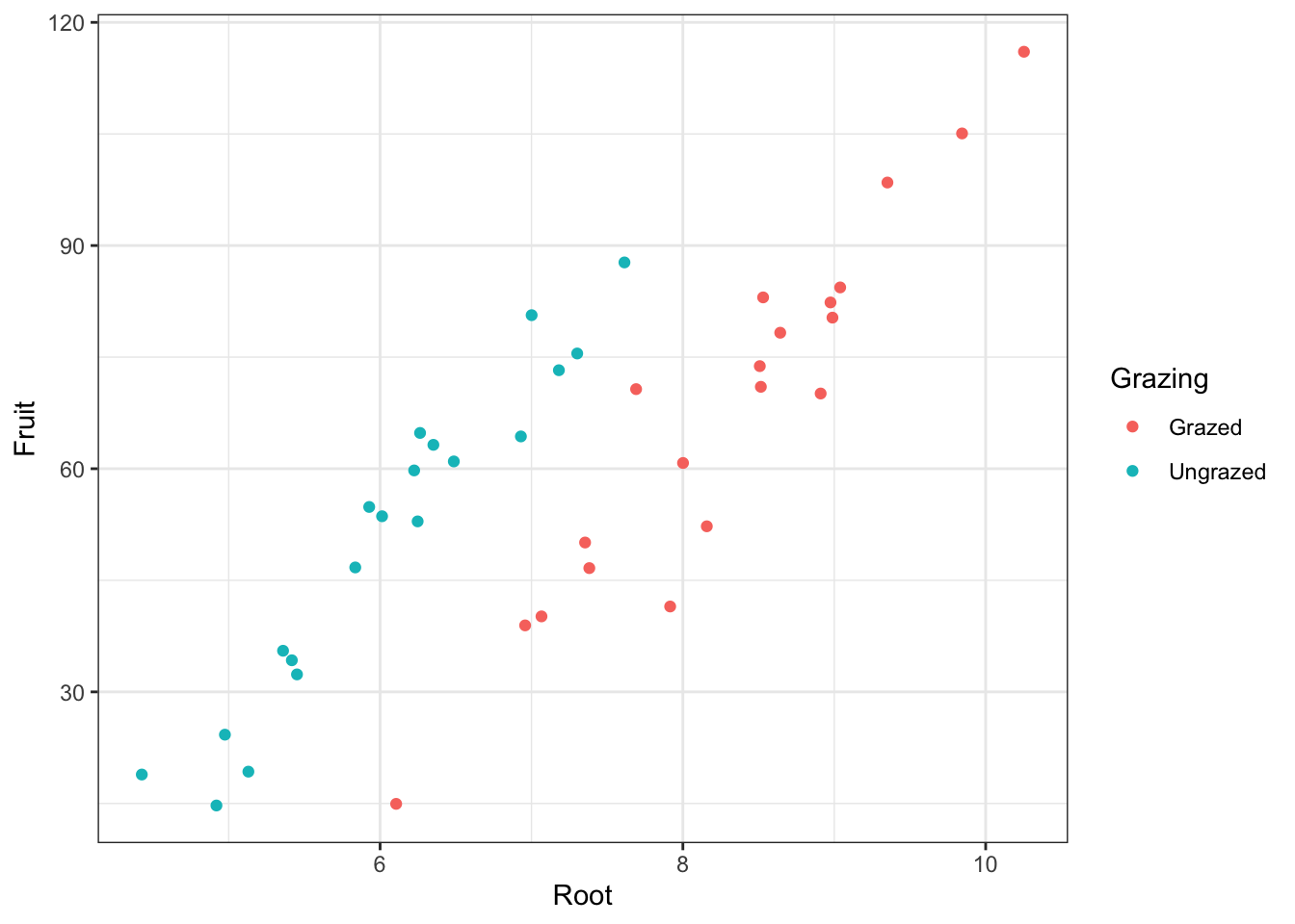

base_plot + 
  theme_bw() + 
  geom_point(
    size = 5) #alter size of datapoints in scatterplot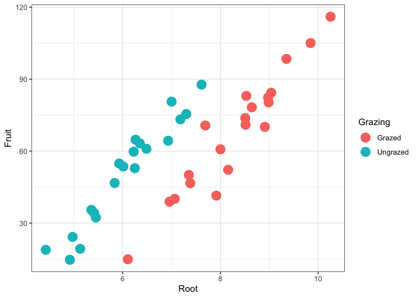 

Add x and y axis titles:

base_plot + theme_bw() + geom_point(size = 5) + 
    xlab("Root Biomass") + 
  ylab("Fruit Production")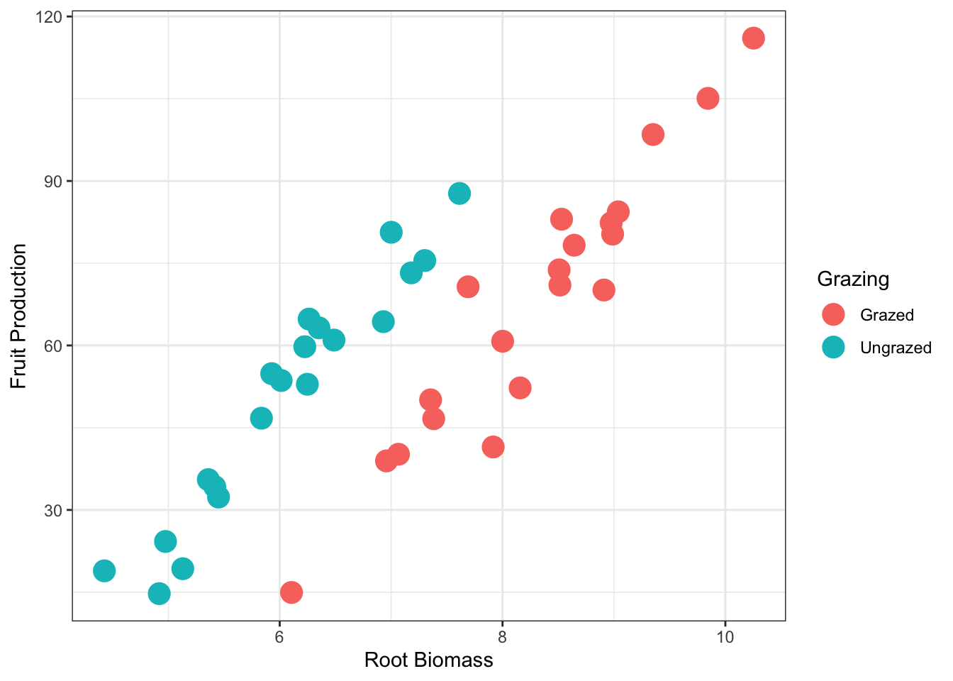 

4.3 Box and whisker plots

base_plot2 <- ggplot(compensation, aes(x = Grazing, y = Fruit)) + 
  geom_boxplot() +  
  geom_point(
    size = 4, #size of point
    colour = 'lightgrey', #color of point
    alpha = 0.5) +         #transparency of point 
  xlab("Grazing treatment") + 
  ylab("Fruit Production") + 
  theme_bw() 
base_plot2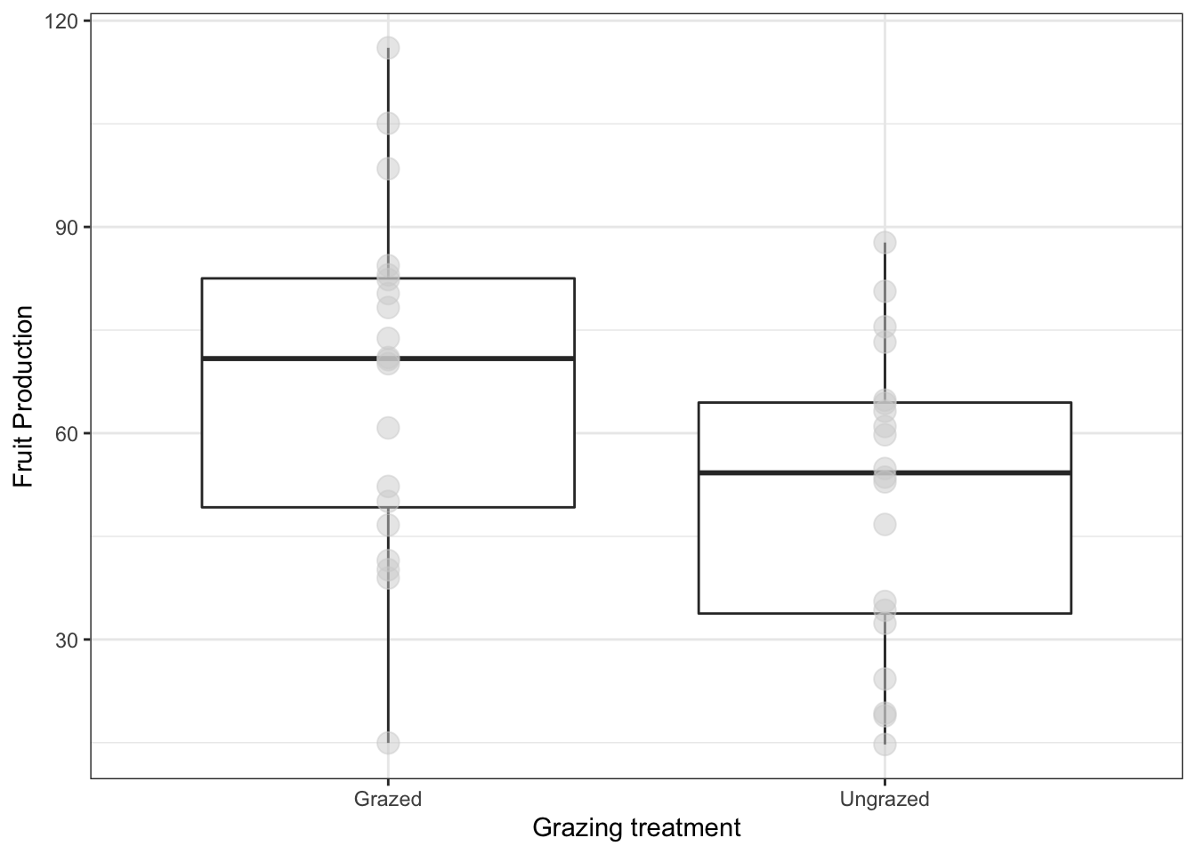

4.4 Distributions: making histograms of numeric variables

ggplot(compensation, aes(x=Fruit))+
  geom_histogram(bins=15)  #bins defines how many histogram bins there are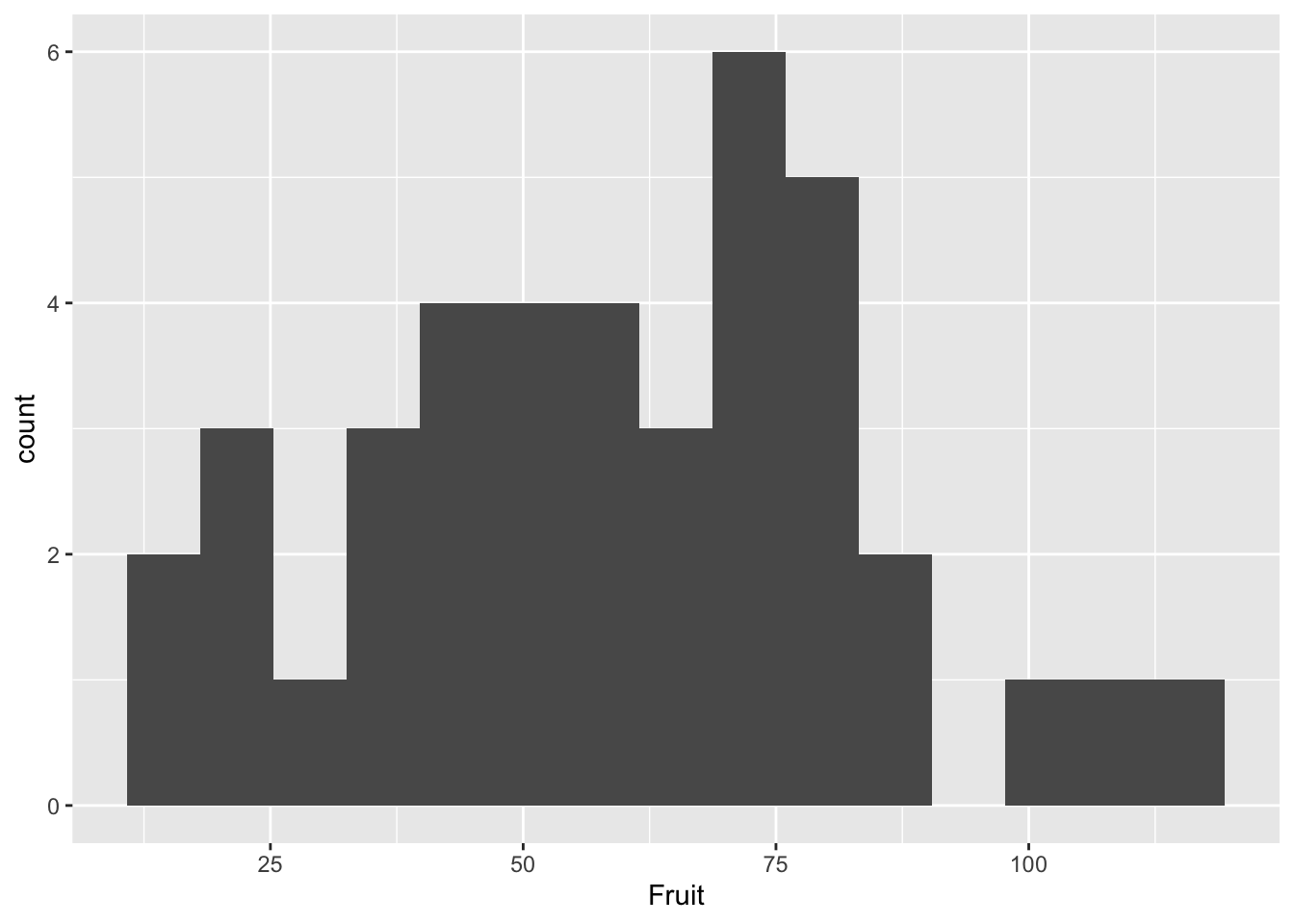 

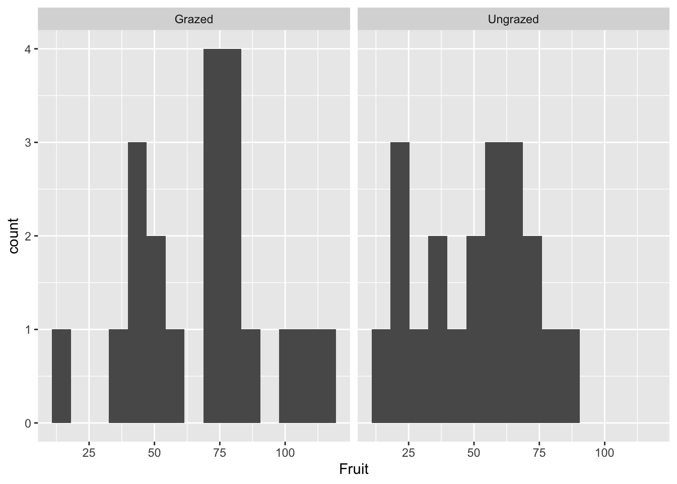
ggplot(compensation, aes(x=Fruit))+
  geom_histogram(bins=15) + 
  facet_wrap(~Grazing) #facet_wrap() allows you to put the plots next to each other, a variable must be specified