6 Variable reconstruction
We now proceed to variable reconstruction where we will take a look at each column separately. While checking every column, we decide whether they will be useful for our analysis and used further or not. However, for the purpose of the project we showcase only the most interesting and especially the most relevant columns to our research questions. If necessary, we will also format, adjust or restructure the data based on the 5 EDA questions, i.e.:
- Is the data correctly formatted?
- Is the data related to our problem?
- Does the data need adjustments?
- Which shape does data exhibit?
- Can we extend the data?
The first column has only 2 unique values - name of the Enterprises - and therefore it should be transformed into a factor
data$`Enterprise Flag` <- as.factor(data$`Enterprise Flag`)
levels(data$`Enterprise Flag`) <- c("Fannie Mae", "Freddie Mac")Desc(data$`Enterprise Flag`)## ----------------------------------------------------------------------------------------------------------------------
## data$`Enterprise Flag` (factor - dichotomous)
##
## length n NAs unique
## 1'000'000 1'000'000 0 2
## 100.0% 0.0%
##
## freq perc lci.95 uci.95'
## Fannie Mae 566'103 56.6% 56.5% 56.7%
## Freddie Mac 433'897 43.4% 43.3% 43.5%
##
## ' 95%-CI (Wilson)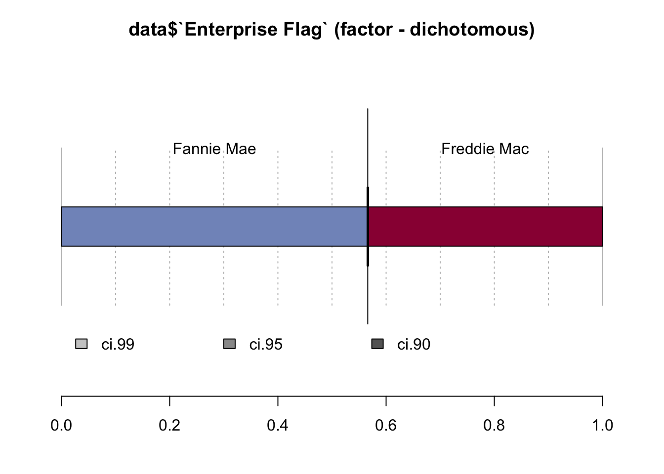
We can observe that there were slightly more mortgage purchases from Fannie Mae company.
The following columns have a specific company-related information and not related to our research. We therefore omit these columns from our data set.
data <- data %>%
  select(-c("Record Number", "Metropolitan Statistical Area (MSA) Code", "County - 2010 Census",
            "Census Tract - 2010 Census", "2010 Census Tract - Percent Minority", "2010 Census Tract - Median Income",
"US Postal State Code"))Desc(data$`Local Area Median Income`)## ----------------------------------------------------------------------------------------------------------------------
## data$`Local Area Median Income` (numeric)
##
## length n NAs unique 0s mean meanCI'
## 1'000'000 999'152 848 1'221 0 75'429.79 75'402.83
## 99.9% 0.1% 0.0% 75'456.75
##
## .05 .10 .25 median .75 .90 .95
## 56'018.00 60'790.00 66'070.00 73'783.00 81'823.00 92'660.00 102'945.00
##
## range sd vcoef mad IQR skew kurt
## 115'261.00 13'748.84 0.18 11'512.39 15'753.00 0.76 0.96
##
## lowest : 18'262.0 (10), 18'943.0 (56), 19'310.0 (27), 19'412.0, 19'903.0 (51)
## highest: 109'946.0 (2'292), 110'923.0 (97), 113'810.0 (22'390), 120'885.0 (4'436), 133'523.0 (84)
##
## ' 95%-CI (classic)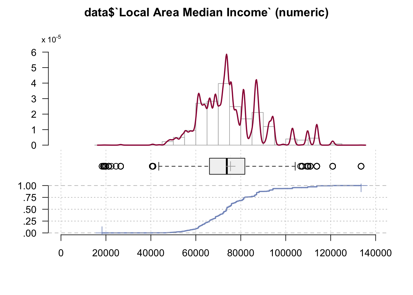
From this graph we can conclude that 75% of the borrowers live in an are with a median income of less than $80000. This is an average income for an American household as it can be observed from the graph.
The Tract Income Ratio is not relevant for us and we therefore omit it.
data <- data %>% select(-`Tract Income Ratio`)Desc(data$`Borrower’s (or Borrowers’) Annual Income`)## ----------------------------------------------------------------------------------------------------------------------
## data$`Borrower’s (or Borrowers’) Annual Income` (numeric)
##
## length n NAs unique 0s mean meanCI'
## 1'000'000 1'000'000 0 1'619 3 131'025.59 123'433.05
## 100.0% 0.0% 0.0% 138'618.13
##
## .05 .10 .25 median .75 .90 .95
## 37'000.00 45'000.00 65'000.00 96'000.00 141'000.00 200'000.00 251'000.00
##
## range sd vcoef mad IQR skew kurt
## 999'999'998.00 3'873'811.67 29.57 53'373.60 76'000.00 257.93 66'571.76
##
## lowest : 0.0 (3), 1'000.0 (6), 2'000.0 (6), 3'000.0 (5), 4'000.0 (7)
## highest: 12'000'000.0 (3), 12'431'000.0, 12'770'000.0, 12'807'000.0, 999'999'998.0 (15)
##
## ' 95%-CI (classic)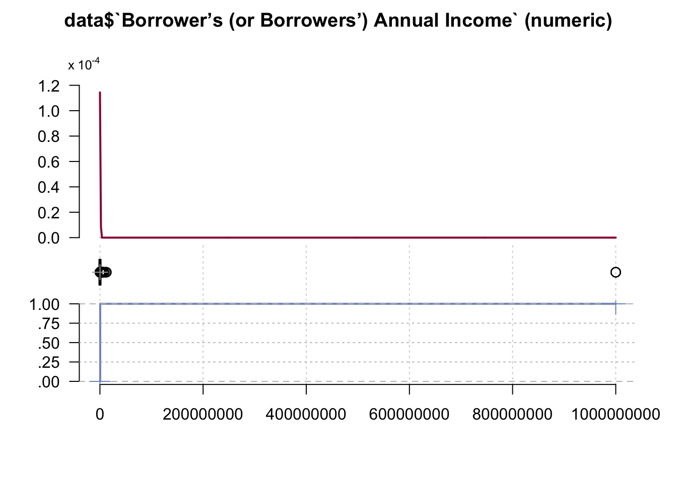
From this graph we may see that there are some outliers (Borrowers with an immense income). We need to get rid of this values to see a clear picture.
data <- subset(data, `Borrower’s (or Borrowers’) Annual Income`!=999999998)Now let’s look at the graph again
Desc(data$`Borrower’s (or Borrowers’) Annual Income`)## ----------------------------------------------------------------------------------------------------------------------
## data$`Borrower’s (or Borrowers’) Annual Income` (numeric)
##
## length n NAs unique 0s mean meanCI'
## 999'985 999'985 0 1'618 3 116'027.33 115'830.28
## 100.0% 0.0% 0.0% 116'224.38
##
## .05 .10 .25 median .75 .90 .95
## 37'000.00 45'000.00 65'000.00 96'000.00 141'000.00 200'000.00 251'000.00
##
## range sd vcoef mad IQR skew kurt
## 12'807'000.00 100'536.92 0.87 53'373.60 76'000.00 23.18 1'994.89
##
## lowest : 0.0 (3), 1'000.0 (6), 2'000.0 (6), 3'000.0 (5), 4'000.0 (7)
## highest: 11'588'000.0, 12'000'000.0 (3), 12'431'000.0, 12'770'000.0, 12'807'000.0
##
## ' 95%-CI (classic)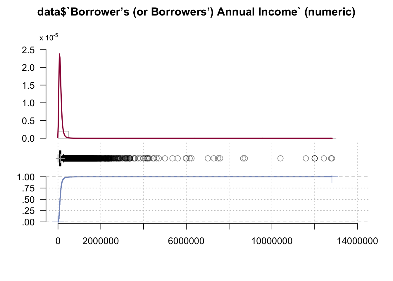
We can observe a high discrepancy overall in the data with 90% of borrower’s having annual income of 200 000 or less.
Desc(data$`Area Median Family Income (2019)`)## ----------------------------------------------------------------------------------------------------------------------
## data$`Area Median Family Income (2019)` (numeric)
##
## length n NAs unique 0s mean meanCI'
## 999'985 999'984 1 421 0 80'343.19 80'313.96
## 100.0% 0.0% 0.0% 80'372.43
##
## .05 .10 .25 median .75 .90 .95
## 58'700.00 64'500.00 69'700.00 79'100.00 87'900.00 99'300.00 109'200.00
##
## range sd vcoef mad IQR skew kurt
## 115'700.00 14'916.70 0.19 13'046.88 18'200.00 0.71 0.85
##
## lowest : 19'800.0 (56), 21'200.0 (27), 21'600.0 (16), 22'200.0 (50), 22'800.0 (16)
## highest: 119'000.0 (2'292), 119'600.0 (13'645), 119'900.0 (22'385), 129'900.0 (4'436), 135'500.0 (84)
##
## ' 95%-CI (classic)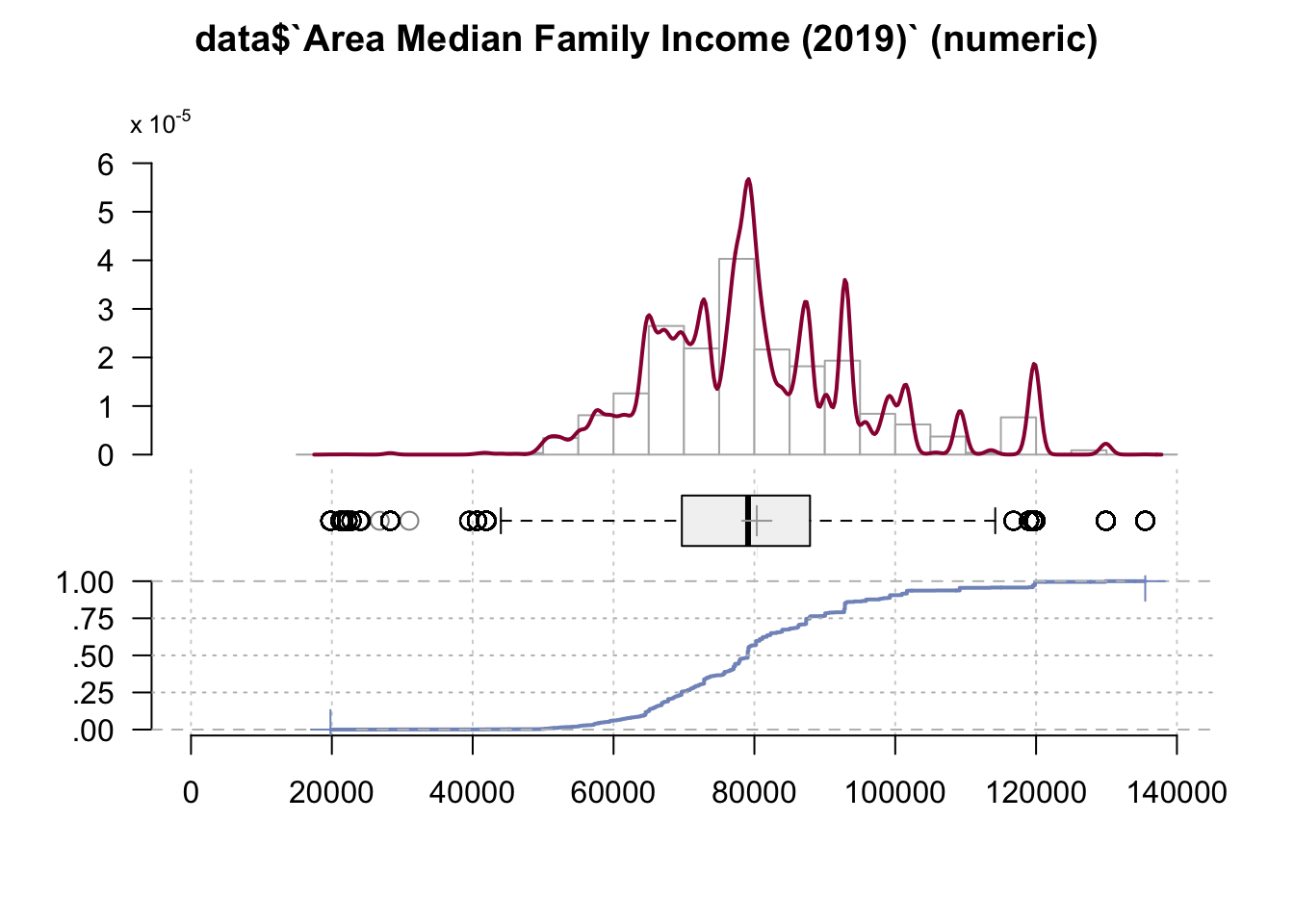
The Area Median Family Income is determined to be at around 80 000 (79 100 to be precise) with half of the observed families earning less than 80 000 and half more than that. We noticed that this variable is almost identical with Local Area Median Income column, therefore we will remove it.
data <- data %>% select(-`Area Median Family Income (2019)`)Desc(data$`Borrower Income Ratio`)## ----------------------------------------------------------------------------------------------------------------------
## data$`Borrower Income Ratio` (numeric)
##
## length n NAs unique 0s mean meanCI'
## 999'985 999'985 0 1'983 3 1.46 1.46
## 100.0% 0.0% 0.0% 1.47
##
## .05 .10 .25 median .75 .90 .95
## 0.48 0.58 0.81 1.20 1.76 2.51 3.19
##
## range sd vcoef mad IQR skew kurt
## 218.17 1.32 0.90 0.65 0.95 26.20 2'544.81
##
## lowest : 0.0 (3), 0.01 (7), 0.02 (4), 0.03 (5), 0.04 (3)
## highest: 159.78, 164.6, 171.17, 172.16, 218.17
##
## ' 95%-CI (classic)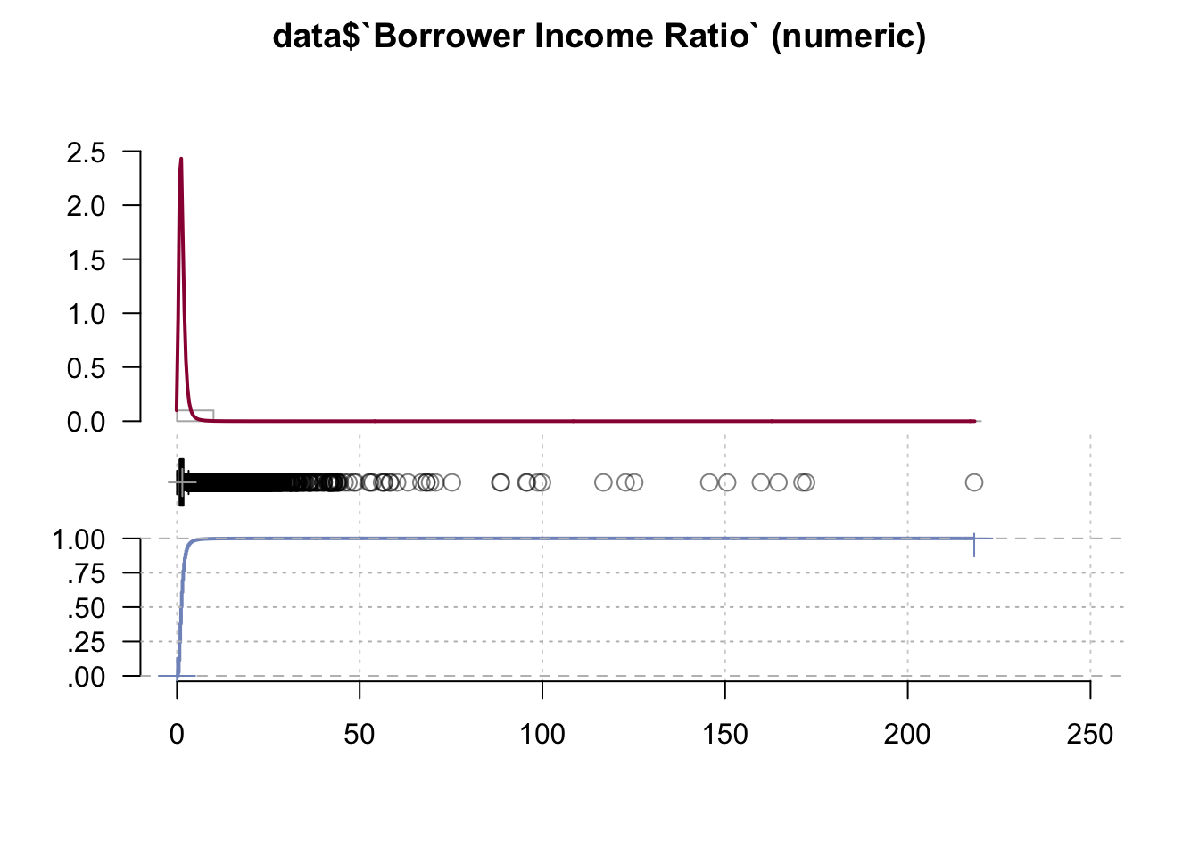
The Borrower Income Ratio shows the ratio of borrower’s annual income to the Area Median Family Income. In this case the graph looks very identical with the ‘Borrower’s annual income’. That is consistent with the column description as this ratio is used to determine the borrower’s qualification.
We further delete Acquisition Unpaid Principal Balance (UPB) as there is no valuable info for us in this column.
data <- data %>% select(-`Acquisition Unpaid Principal Balance (UPB)`)Then, in the description file we noticed that some of our columns (e.g. Purpose of Loan, Borrower Race, Borrower Ethnicity etc.) are encoded. So, we can conclude that these columns contain categorical data and thus should be transformed into factors and the respective levels should be determined.
data$`Purpose of Loan` <- as.factor(data$`Purpose of Loan`)
data$`First-Time Home Buyer` <- as.factor(data$`First-Time Home Buyer`)
data$`Borrower Race1` <- as.factor(data$`Borrower Race1`)
data$`Co-Borrower Race1` <- as.factor(data$`Co-Borrower Race1`)
data$`Borrower Gender` <- as.factor(data$`Borrower Gender`)
data$`Co-Borrower Gender` <- as.factor(data$`Co-Borrower Gender`)
data$`Age of Borrower` <- as.factor(data$`Age of Borrower`)
data$`Age of Co-Borrower` <- as.factor(data$`Age of Co-Borrower`)
data$`Occupancy Code` <- as.factor(data$`Occupancy Code`)
data$`Property Type` <- as.factor(data$`Property Type`)
data$`Date of Mortgage Note` <- as.factor(data$`Date of Mortgage Note`)
data$`Persistent Poverty County` <- as.factor(data$`Persistent Poverty County`)
data$`Area of Concentrated Poverty` <- as.factor(data$`Area of Concentrated Poverty`)
data$`High Opportunity Area` <- as.factor(data$`High Opportunity Area`)
Now we need to decipher our encoded columns. We will do this by defining levels of the columns which we transformed into factors.
levels(data$`Purpose of Loan`) <- c(1, 2, 4, 7)
levels(data$`Purpose of Loan`) <- c("Purchase", "Refinancing", "Home improvement", "Refinancing cash-out")

levels(data$`First-Time Home Buyer`) <- c(1, 2)
levels(data$`First-Time Home Buyer`) <- c("Yes", "No")

levels(data$`Borrower Race1`) <- c(1, 2, 3, 4, 5)
levels(data$`Borrower Race1`) <- c("American Indian or Alaska Native", "Asian", "Black or African American",
                                   "Native Hawaiian or Other Pacific Islander", "White")

levels(data$`Co-Borrower Race1`) <- c(1, 2, 3, 4, 5)
levels(data$`Co-Borrower Race1`) <- c("American Indian or Alaska Native", "Asian", "Black or African American",
                                   "Native Hawaiian or Other Pacific Islander", "White", "no co-borrower")

levels(data$`Borrower Gender`) <- c(1, 2)
levels(data$`Borrower Gender`) <- c("Male", "Female")

levels(data$`Co-Borrower Gender`) <- c(1, 2)
levels(data$`Co-Borrower Gender`) <- c("Male", "Female")

levels(data$`Age of Borrower`) <- c(1, 2, 3, 4, 5, 6, 7)
levels(data$`Age of Borrower`) <- c("under 25 years old", "25 to 34 years old", "35 to 44 years old",
                                    "45 to 54 years old", "55 to 64 years old", "65 to 74 years old",
                                    "over 74 years old")

levels(data$`Age of Co-Borrower`) <- c(1, 2, 3, 4, 5, 6, 7)
levels(data$`Age of Co-Borrower`) <- c("under 25 years old", "25 to 34 years old", "35 to 44 years old",
                                    "45 to 54 years old", "55 to 64 years old", "65 to 74 years old",
                                    "over 74 years old")

levels(data$`Occupancy Code`) <- c(1, 2, 3)
levels(data$`Occupancy Code`) <- c("Principal Residence/Owner-Occupied property", "Second Home", "Investment property")

levels(data$`Property Type`) <- c(1, 2)
levels(data$`Property Type`) <- c("one to four-family (other than manufactured housing)", "manufactured housing")

levels(data$`Date of Mortgage Note`) <- c(1, 2)
levels(data$`Date of Mortgage Note`) <- c("Originated in same calendar year as acquired",
                                          "Originated prior to calendar year of acquisition")

levels(data$`Persistent Poverty County`) <- c(0, 1)
levels(data$`Persistent Poverty County`) <- c("No", "Yes")

levels(data$`Area of Concentrated Poverty`) <- c(0, 1)
levels(data$`Area of Concentrated Poverty`) <- c("No", "Yes")

levels(data$`High Opportunity Area`) <- c(0, 1)
levels(data$`High Opportunity Area`) <- c("No", "Yes")
Now we can make further analysis.
Desc(data$`Purpose of Loan`)## ----------------------------------------------------------------------------------------------------------------------
## data$`Purpose of Loan` (factor)
##
## length n NAs unique levels dupes
## 999'985 999'985 0 4 4 y
## 100.0% 0.0%
##
## level freq perc cumfreq cumperc
## 1 Purchase 544'618 54.5% 544'618 54.5%
## 2 Refinancing 242'591 24.3% 787'209 78.7%
## 3 Refinancing cash-out 212'241 21.2% 999'450 99.9%
## 4 Home improvement 535 0.1% 999'985 100.0%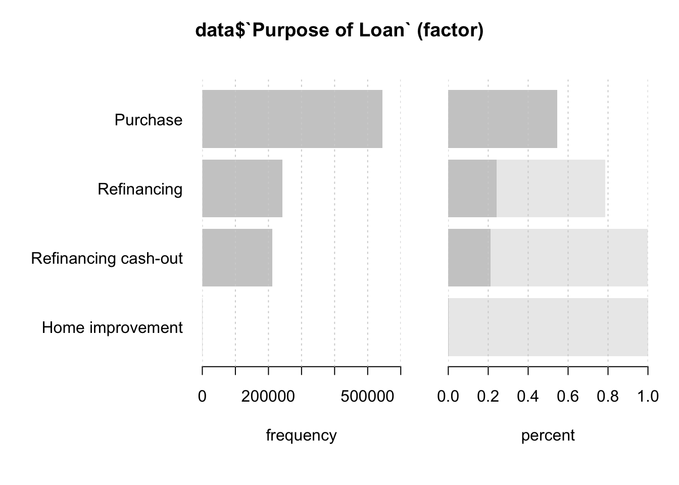
From this table we can instantly see that the majority of loans are used for a home purchase. This could be useful for the further analysis reagrding social and economical factors having influence on mortgage amount.
We further delete Federal Guarantee column from our data set.
data <- data %>% select(-`Federal Guarantee`)Desc(data$`Number of Borrowers`)## ----------------------------------------------------------------------------------------------------------------------
## data$`Number of Borrowers` (numeric)
##
## length n NAs unique 0s mean meanCI'
## 999'985 999'985 0 6 0 1.47 1.47
## 100.0% 0.0% 0.0% 1.47
##
## .05 .10 .25 median .75 .90 .95
## 1.00 1.00 1.00 1.00 2.00 2.00 2.00
##
## range sd vcoef mad IQR skew kurt
## 5.00 0.51 0.35 0.00 1.00 0.30 -1.30
##
##
## value freq perc cumfreq cumperc
## 1 1 535'281 53.5% 535'281 53.5%
## 2 2 459'355 45.9% 994'636 99.5%
## 3 3 4'630 0.5% 999'266 99.9%
## 4 4 716 0.1% 999'982 100.0%
## 5 5 2 0.0% 999'984 100.0%
## 6 6 1 0.0% 999'985 100.0%
##
## ' 95%-CI (classic)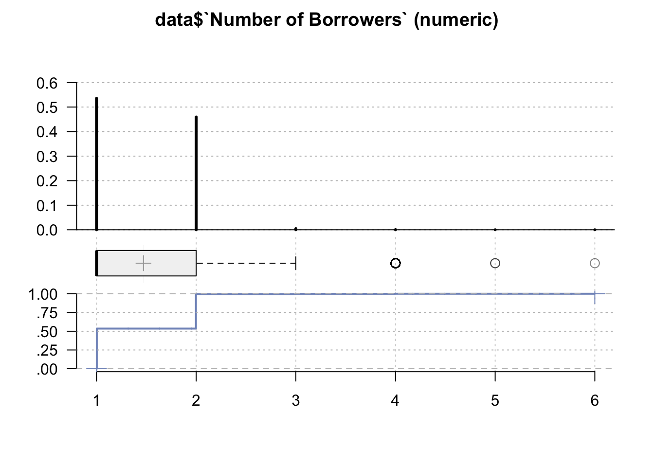
Values 3-6 can be considered outliers, almost all the mortgages were signed by either 1 or 2 persons.
Desc(data$`First-Time Home Buyer`)## ----------------------------------------------------------------------------------------------------------------------
## data$`First-Time Home Buyer` (factor - dichotomous)
##
## length n NAs unique
## 999'985 999'720 265 2
## 100.0% 0.0%
##
## freq perc lci.95 uci.95'
## Yes 232'398 23.2% 23.2% 23.3%
## No 767'322 76.8% 76.7% 76.8%
##
## ' 95%-CI (Wilson)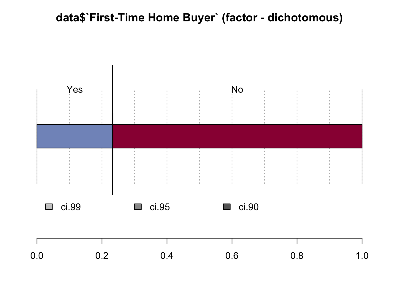
A significant majority of borrowers are not first-time home buyers, which together with Purpose of Loan indicates that most of the borrowers purchase more homes for whatever reasons, but not for the first time.
For the simplicity, we also rename the Borrower Race column.
data <- data %>% rename("Borrower Race" = `Borrower Race1`)Desc(data$`Borrower Race`)## ----------------------------------------------------------------------------------------------------------------------
## data$`Borrower Race` (factor)
##
## length n NAs unique levels dupes
## 999'985 858'248 141'737 5 5 y
## 85.8% 14.2%
##
## level freq perc cumfreq cumperc
## 1 White 742'115 86.5% 742'115 86.5%
## 2 Asian 70'216 8.2% 812'331 94.6%
## 3 Black or African American 39'137 4.6% 851'468 99.2%
## 4 American Indian or Alaska Native 4'341 0.5% 855'809 99.7%
## 5 Native Hawaiian or Other Pacific Islander 2'439 0.3% 858'248 100.0%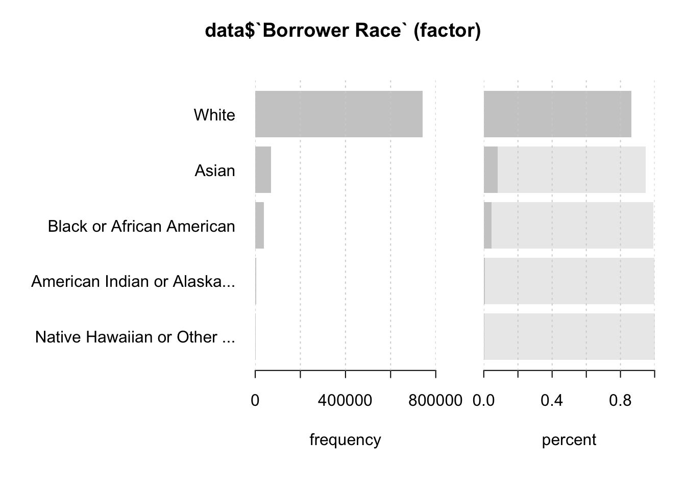
We can observe that most of the companies’ borrowers consist of white people followed by Asians. We could further examine as to why it is so, whether mostly white people applied or because other races were declined.
Further, borrower and co-borrower ethnicity gives us very little information so we drop these columns.
data <- data %>% select(-`Borrower Ethnicity`)
data <- data %>% select(-`Co-Borrower Ethnicity`)
We also rename the Co-Borrower's Race1 column
data <- data %>% rename("Co-Borrower Race" = `Co-Borrower Race1`)Desc(data$`Co-Borrower Race` )## ----------------------------------------------------------------------------------------------------------------------
## data$`Co-Borrower Race` (factor)
##
## length n NAs unique levels dupes
## 999'985 397'213 602'772 5 6 y
## 39.7% 60.3%
##
## level freq perc cumfreq cumperc
## 1 White 352'092 88.6% 352'092 88.6%
## 2 Asian 30'770 7.7% 382'862 96.4%
## 3 Black or African American 11'001 2.8% 393'863 99.2%
## 4 American Indian or Alaska Native 2'105 0.5% 395'968 99.7%
## 5 Native Hawaiian or Other Pacific Islander 1'245 0.3% 397'213 100.0%
## 6 no co-borrower 0 0.0% 397'213 100.0%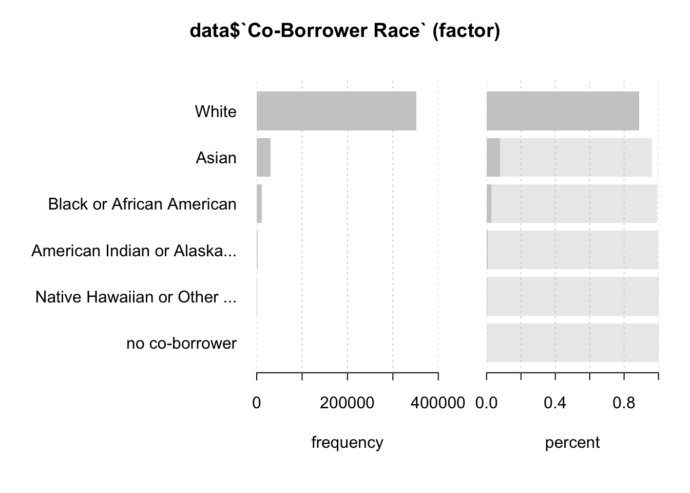
The data is very much identical to Borrower's Race indicating that the proportion is the same.
Desc(data$`Borrower Gender`)## ----------------------------------------------------------------------------------------------------------------------
## data$`Borrower Gender` (factor - dichotomous)
##
## length n NAs unique
## 999'985 920'376 79'609 2
## 92.0% 8.0%
##
## freq perc lci.95 uci.95'
## Male 612'829 66.6% 66.5% 66.7%
## Female 307'547 33.4% 33.3% 33.5%
##
## ' 95%-CI (Wilson)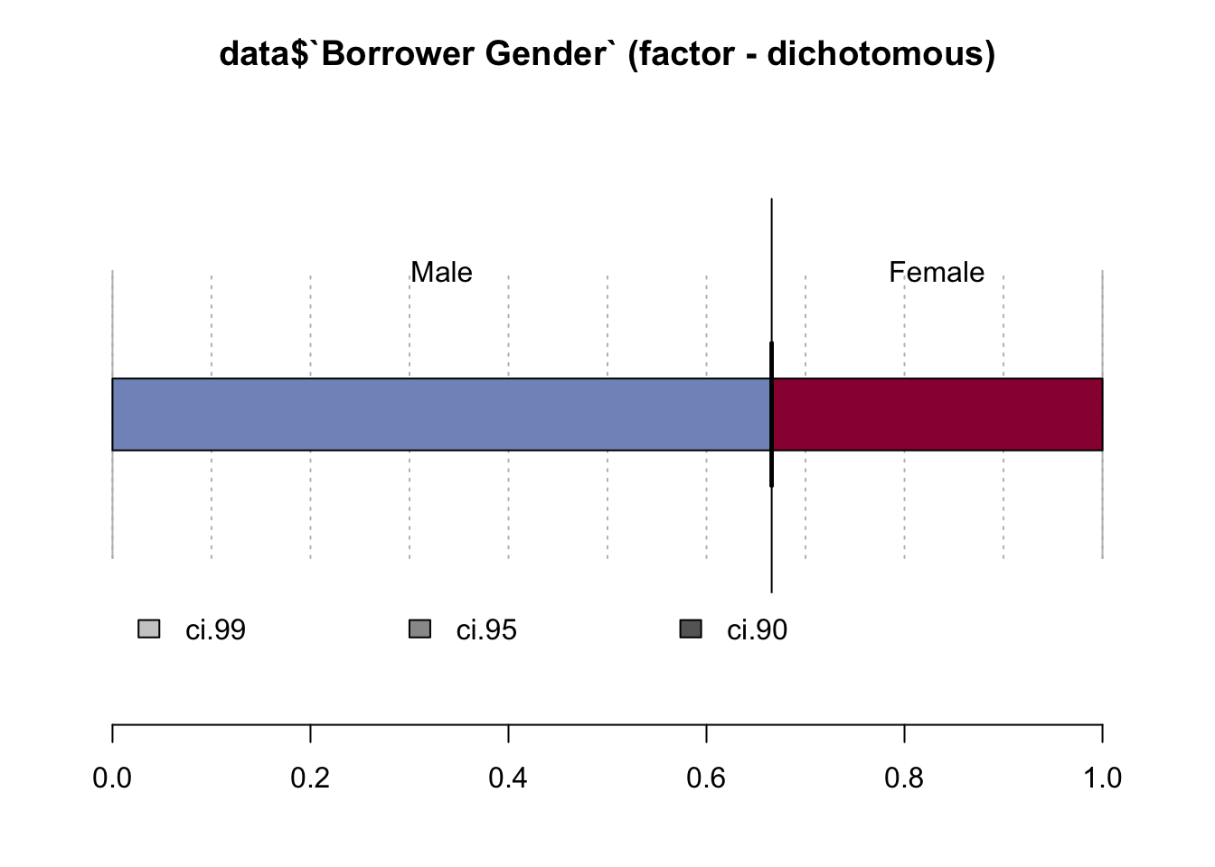
The main borrower is in 67% of all cases a male.
Desc(data$`Co-Borrower Gender`)## ----------------------------------------------------------------------------------------------------------------------
## data$`Co-Borrower Gender` (factor - dichotomous)
##
## length n NAs unique
## 999'985 424'443 575'542 2
## 42.4% 57.6%
##
## freq perc lci.95 uci.95'
## Male 107'228 25.3% 25.1% 25.4%
## Female 317'215 74.7% 74.6% 74.9%
##
## ' 95%-CI (Wilson)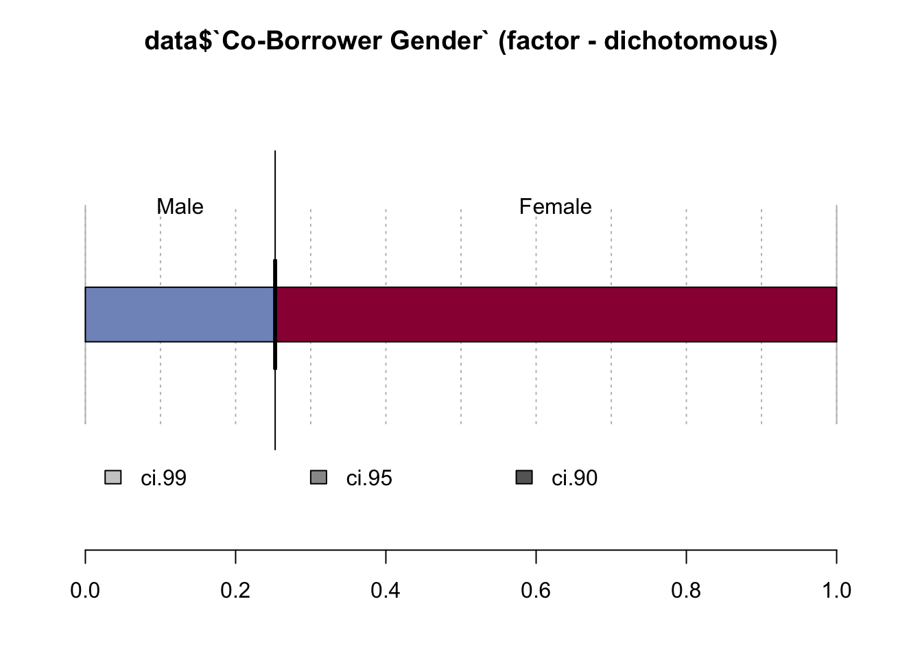
However, the co-borrower tends to be in 75% of all cases a woman. That could mean that couples co-apply.
Desc(data$`Age of Borrower`)## ----------------------------------------------------------------------------------------------------------------------
## data$`Age of Borrower` (factor)
##
## length n NAs unique levels dupes
## 999'985 999'960 25 7 7 y
## 100.0% 0.0%
##
## level freq perc cumfreq cumperc
## 1 35 to 44 years old 257'033 25.7% 257'033 25.7%
## 2 25 to 34 years old 231'205 23.1% 488'238 48.8%
## 3 45 to 54 years old 211'435 21.1% 699'673 70.0%
## 4 55 to 64 years old 164'166 16.4% 863'839 86.4%
## 5 65 to 74 years old 85'732 8.6% 949'571 95.0%
## 6 under 25 years old 26'501 2.7% 976'072 97.6%
## 7 over 74 years old 23'888 2.4% 999'960 100.0%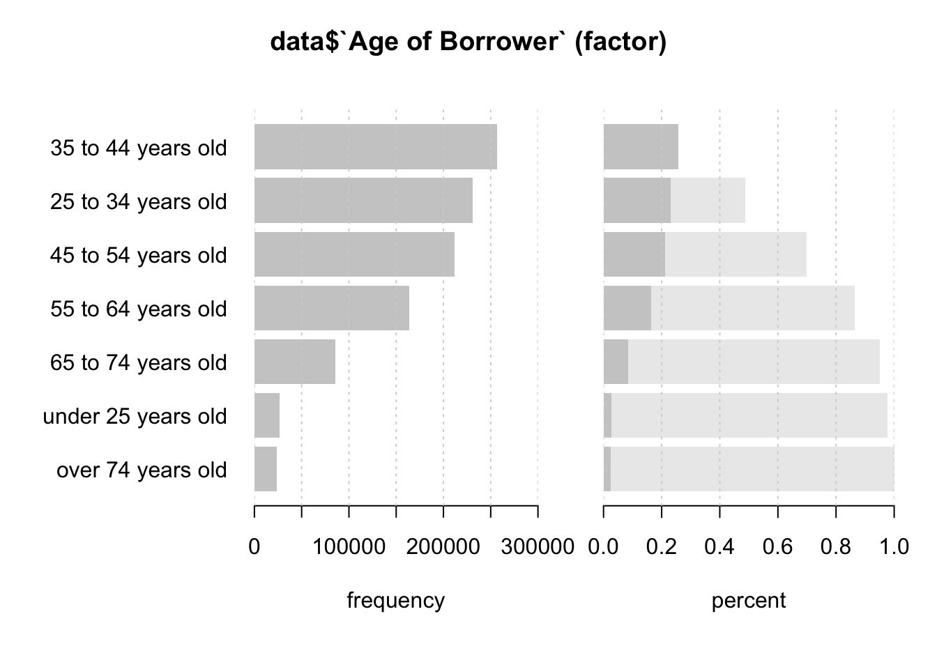
The Age of Borrower gives us a good overview of the age distribution. Three age groups stand out the most: 35-44, 25-34, and 45-54.
Desc(data$`Age of Co-Borrower`)## ----------------------------------------------------------------------------------------------------------------------
## data$`Age of Co-Borrower` (factor)
##
## length n NAs unique levels dupes
## 999'985 464'687 535'298 7 7 y
## 46.5% 53.5%
##
## level freq perc cumfreq cumperc
## 1 35 to 44 years old 115'052 24.8% 115'052 24.8%
## 2 25 to 34 years old 109'971 23.7% 225'023 48.4%
## 3 45 to 54 years old 93'271 20.1% 318'294 68.5%
## 4 55 to 64 years old 80'302 17.3% 398'596 85.8%
## 5 65 to 74 years old 44'432 9.6% 443'028 95.3%
## 6 under 25 years old 11'067 2.4% 454'095 97.7%
## 7 over 74 years old 10'592 2.3% 464'687 100.0%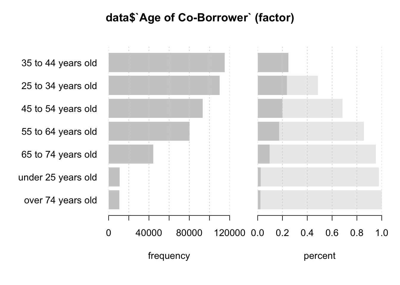
The data in this column is again very much identical to the previous one.
Desc(data$`Occupancy Code`)## ----------------------------------------------------------------------------------------------------------------------
## data$`Occupancy Code` (factor)
##
## length n NAs unique levels dupes
## 999'985 999'985 0 3 3 y
## 100.0% 0.0%
##
## level freq perc cumfreq cumperc
## 1 Principal Residence/Owner-Occupied property 897'838 89.8% 897'838 89.8%
## 2 Investment property 61'468 6.1% 959'306 95.9%
## 3 Second Home 40'679 4.1% 999'985 100.0%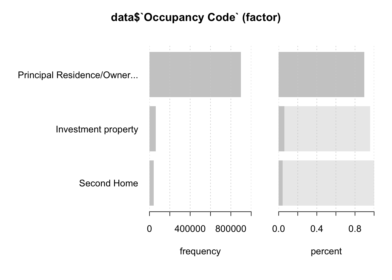
An owner-occupied property is a piece of real estate in which the person who holds the title (or owns the property) also uses the home as their primary residence. The term “owner-occupied” is commonly associated with real estate investors who live in a property and rent out separate spaces to tenants. Here we can observe that vast majority of the borrowers obtained a loan for their own property and their own house usage.
Columns Rate Spread, HOEPA Status, Lien Status are already deleted, as there was a high percentage of missing values.
Desc(data$`Property Type`)## ----------------------------------------------------------------------------------------------------------------------
## data$`Property Type` (factor - dichotomous)
##
## length n NAs unique
## 999'985 999'985 0 2
## 100.0% 0.0%
##
## freq perc lci.95 uci.95'
## one to four-family (other than manufactured housing) 993'218 99.3% 99.3% 99.3%
## manufactured housing 6'767 0.7% 0.7% 0.7%
##
## ' 95%-CI (Wilson)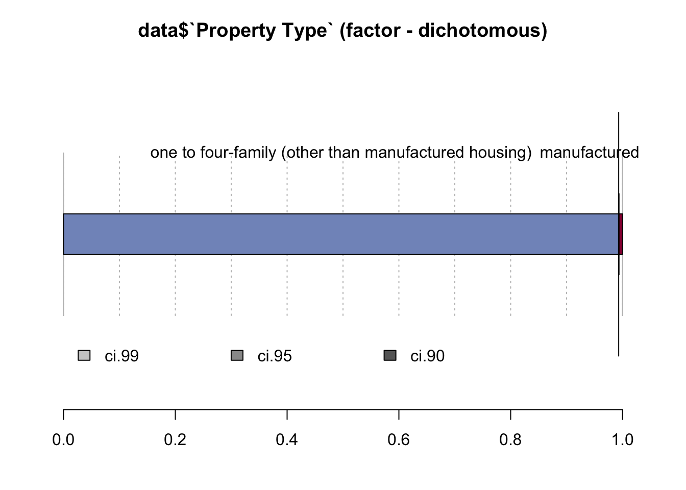
Almost 100% are one to four meaning that this is an ordinary house that is being mortgaged.
The next columns are useless because we already have this information from Age of Borrower
data <- data %>% select(-`Borrower Age 62 or older`)
data <- data %>% select(-`Co-Borrower Age 62 or older`)Desc(data$`Loan-to-Value Ratio (LTV)`)## ----------------------------------------------------------------------------------------------------------------------
## data$`Loan-to-Value Ratio (LTV)` (numeric)
##
## length n NAs unique 0s mean meanCI'
## 999'985 999'982 3 9'164 0 75.62 75.58
## 100.0% 0.0% 0.0% 75.65
##
## .05 .10 .25 median .75 .90 .95
## 41.00 51.00 67.34 80.00 90.00 95.00 97.00
##
## range sd vcoef mad IQR skew kurt
## 304.77 17.12 0.23 14.83 22.66 -0.96 0.80
##
## lowest : 3.23, 3.5, 3.82, 3.91, 4.0 (3)
## highest: 159.0, 162.0, 200.0, 203.0, 308.0
##
## heap(?): remarkable frequency (18.6%) for the mode(s) (= 80)
##
## ' 95%-CI (classic)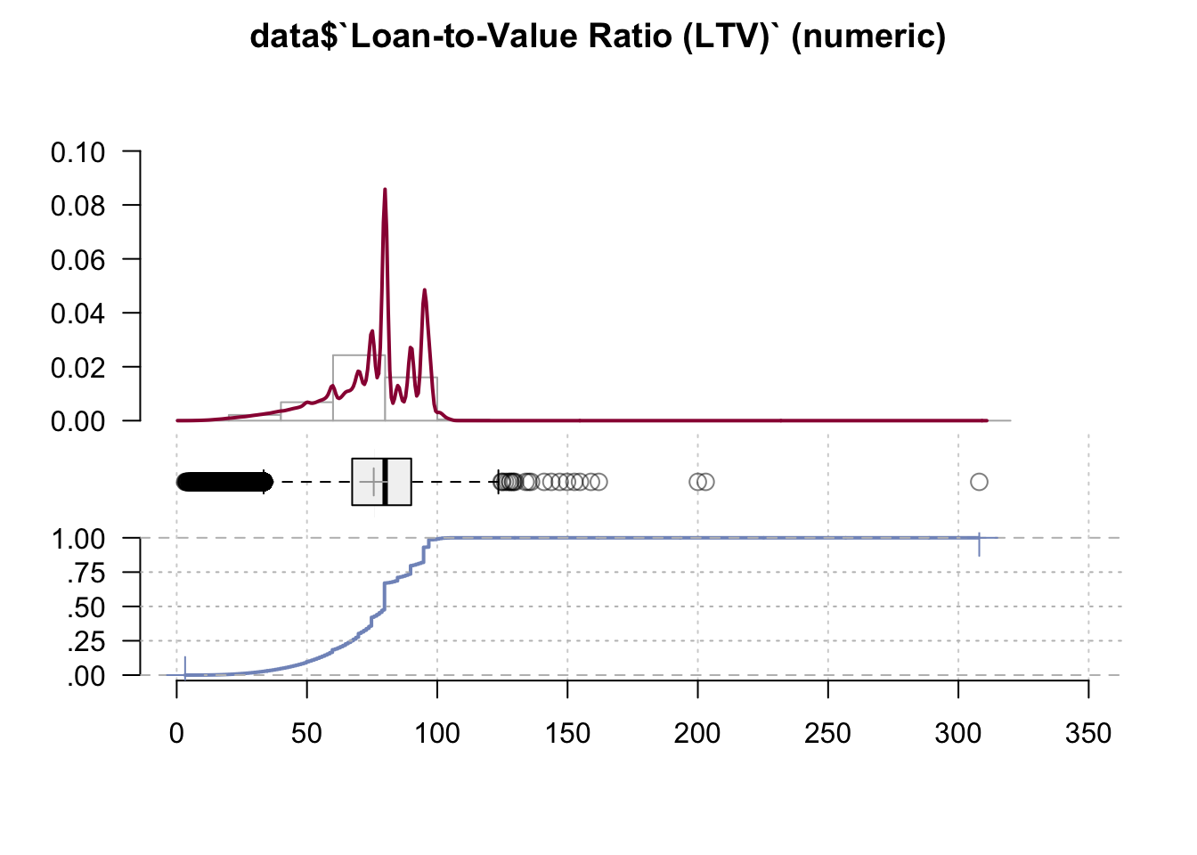
We can observe two spikes, one at 80 and a smaller one at around 100. Generally speaking, most lenders consider a LTV of 80% or more as being risky. If the LTV is higher than 80%, you may need to pay for Lenders Mortgage Insurance Therefore, from this line graph we may conclude that LTV Ratio indicates no or very little risk in all cases.
Desc(data$`Date of Mortgage Note`)## ----------------------------------------------------------------------------------------------------------------------
## data$`Date of Mortgage Note` (factor - dichotomous)
##
## length n NAs unique
## 999'985 999'985 0 2
## 100.0% 0.0%
##
## freq perc lci.95 uci.95'
## Originated in same calendar year as acquired 900'004 90.0% 89.9% 90.1%
## Originated prior to calendar year of acquisition 99'981 10.0% 9.9% 10.1%
##
## ' 95%-CI (Wilson)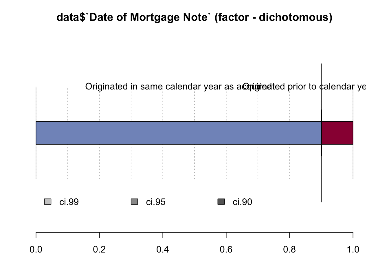
Here we see that mostly mortgage note was originated at the same calendar year.
Desc(data$`Term of Mortgage at Origination`)## ----------------------------------------------------------------------------------------------------------------------
## data$`Term of Mortgage at Origination` (numeric)
##
## length n NAs unique 0s mean meanCI'
## 999'985 999'985 0 156 0 332.48 332.35
## 100.0% 0.0% 0.0% 332.60
##
## .05 .10 .25 median .75 .90 .95
## 180.00 180.00 360.00 360.00 360.00 360.00 360.00
##
## range sd vcoef mad IQR skew kurt
## 420.00 63.21 0.19 0.00 0.00 -1.96 2.07
##
## lowest : 60.0 (4), 84.0 (5), 85.0, 96.0 (264), 102.0
## highest: 357.0 (15), 358.0 (25), 359.0 (35), 360.0 (832'505), 480.0 (3)
##
## heap(?): remarkable frequency (83.3%) for the mode(s) (= 360)
##
## ' 95%-CI (classic)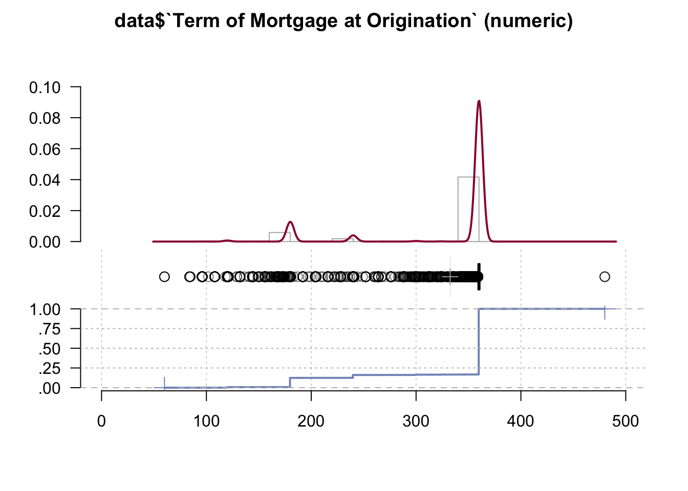
The term of your mortgage loan is how long you have to repay the loan. For most types of homes, mortgage terms are typically 15, 20 or 30 years. On average mortgage is given for 30 years in our case.
Desc(data$`Number of Units`)## ----------------------------------------------------------------------------------------------------------------------
## data$`Number of Units` (numeric)
##
## length n NAs unique 0s mean meanCI'
## 999'985 999'985 0 4 0 1.02 1.02
## 100.0% 0.0% 0.0% 1.02
##
## .05 .10 .25 median .75 .90 .95
## 1.00 1.00 1.00 1.00 1.00 1.00 1.00
##
## range sd vcoef mad IQR skew kurt
## 3.00 0.21 0.20 0.00 0.00 10.27 120.96
##
##
## value freq perc cumfreq cumperc
## 1 1 982'421 98.2% 982'421 98.2%
## 2 2 12'740 1.3% 995'161 99.5%
## 3 3 2'692 0.3% 997'853 99.8%
## 4 4 2'132 0.2% 999'985 100.0%
##
## ' 95%-CI (classic)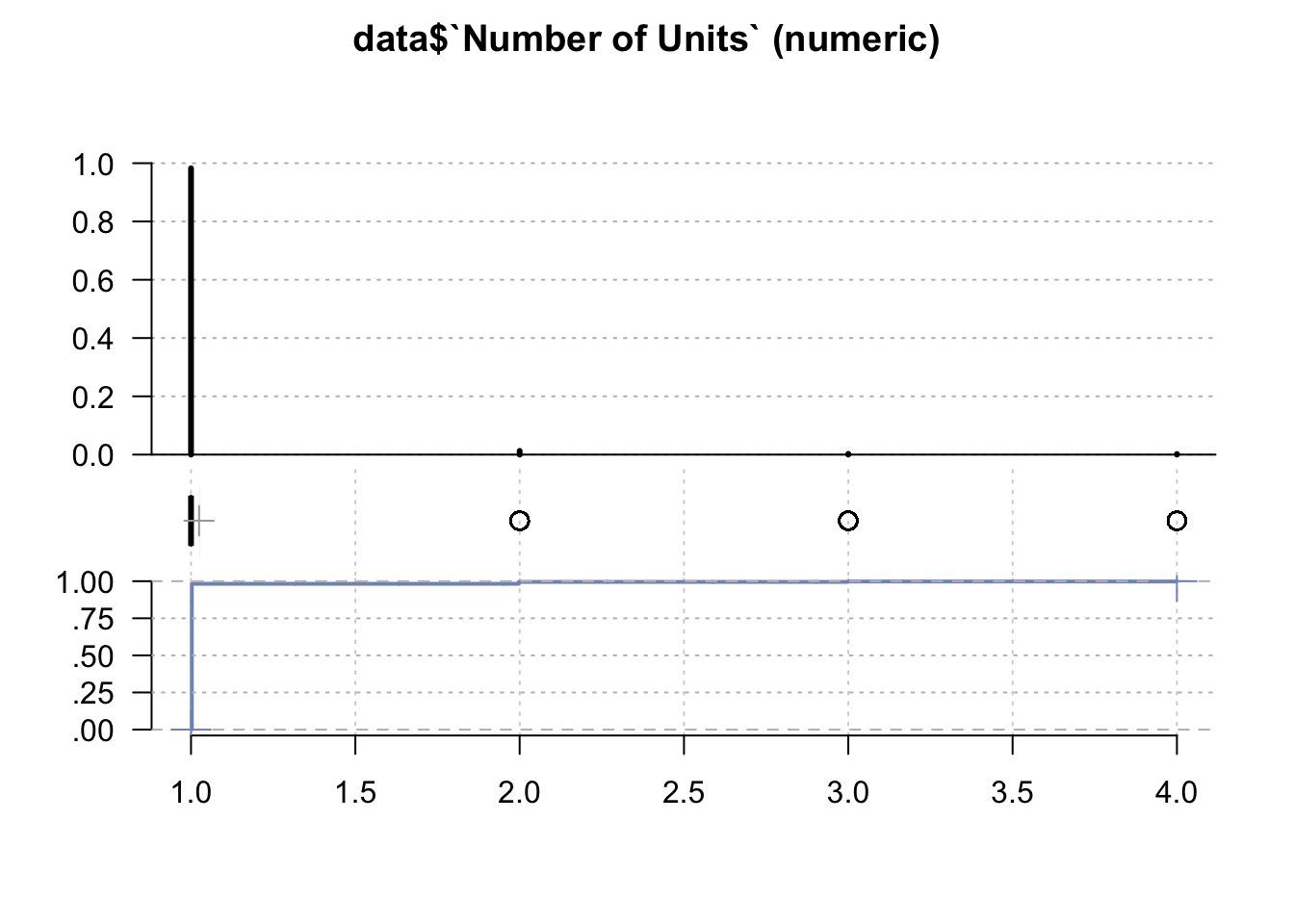
A 2-4 unit property, sometimes referred to as a “triplex” or “fourplex,” has two or three available units to rent out. This is different than having a spare room, or a basement with a kitchenette. A true 2-4 unit property contains legally separate units. Single-unit properties are any properties in which you have a single bookable unit, be it a house, a villa, or a condo.
So, we may see that the result correlates with the previous finding - almost in 100% borrower takes a mortgage for yourself.
Desc(data$`Interest Rate at Origination`)## ----------------------------------------------------------------------------------------------------------------------
## data$`Interest Rate at Origination` (numeric)
##
## length n NAs unique 0s mean meanCI'
## 999'985 999'911 74 366 0 4.24 4.24
## 100.0% 0.0% 0.0% 4.24
##
## .05 .10 .25 median .75 .90 .95
## 3.37 3.50 3.87 4.12 4.62 5.00 5.37
##
## range sd vcoef mad IQR skew kurt
## 7.93 0.62 0.15 0.56 0.75 0.51 0.22
##
## lowest : 0.62, 2.0 (2), 2.12 (4), 2.25 (28), 2.37 (81)
## highest: 7.25 (3), 7.37 (2), 7.62 (2), 7.87 (2), 8.55
##
## heap(?): remarkable frequency (10.1%) for the mode(s) (= 3.87)
##
## ' 95%-CI (classic)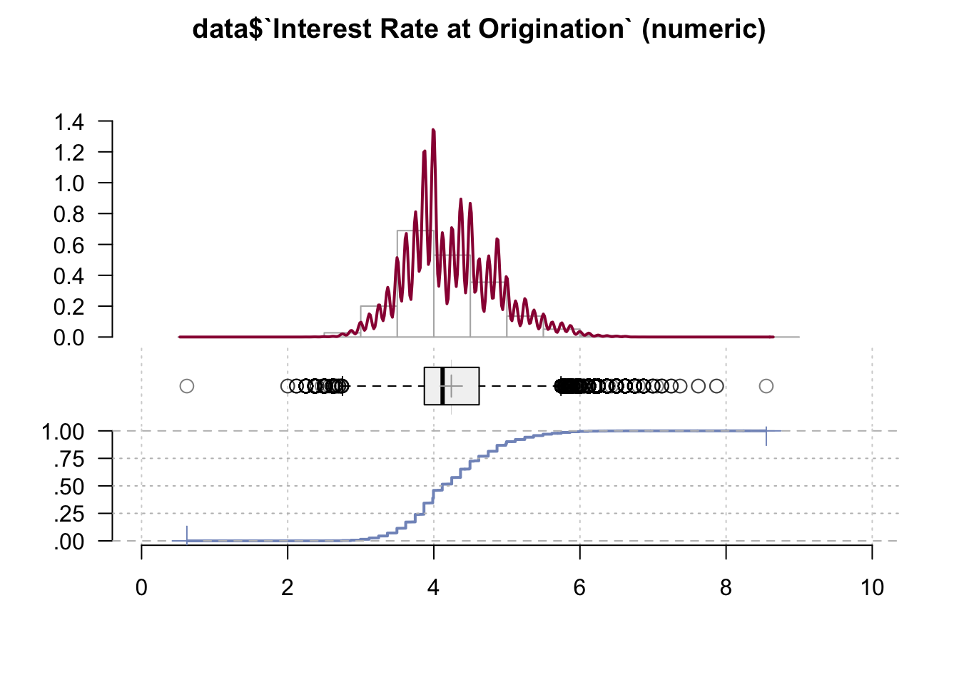
We can observe that Interest Rate at Origination follows several spikes. Interest Rate at Origination is perhaps grouped into several categories, which could explain the observed frequency.
Desc(data$`Note Amount`)## ----------------------------------------------------------------------------------------------------------------------
## data$`Note Amount` (numeric)
##
## length n NAs unique 0s mean meanCI'
## 999'985 999'911 74 130 0 260'105.87 259'847.26
## 100.0% 0.0% 0.0% 260'364.49
##
## .05 .10 .25 median .75 .90 .95
## 85'000.00 105'000.00 155'000.00 235'000.00 345'000.00 445'000.00 485'000.00
##
## range sd vcoef mad IQR skew kurt
## 1'390'000.00 131'944.64 0.51 133'434.00 190'000.00 0.82 0.66
##
## lowest : 5'000.0, 15'000.0 (77), 25'000.0 (607), 35'000.0 (1'899), 45'000.0 (4'108)
## highest: 1'355'000.0, 1'365'000.0, 1'375'000.0, 1'385'000.0, 1'395'000.0 (2)
##
## ' 95%-CI (classic)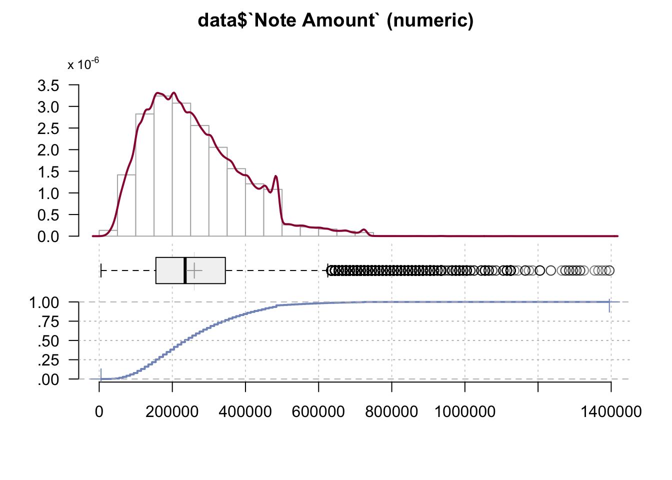
Note Amount refers to the money lent. Note Amount is a part of a mortgage note, which is a written promise to repay a specified sum of money plus interest at a specified rate and length of time to fulfill the promise. The graph displays many outliers - borrowers with extraordinarily high note amounts. We are interested to find out if these individuals also had the highest income.
We delete the following columns as they need more expertise or company-specific info
data <- data %>% select(-c("Preapproval", "Application Channel", "Automated Underwriting System (AUS)",
"Credit Score Model - Borrower", "Credit Score Model - Co-Borrower"))Desc(data$`Debt-to-Income (DTI) Ratio`)## ----------------------------------------------------------------------------------------------------------------------
## data$`Debt-to-Income (DTI) Ratio` (numeric)
##
## length n NAs unique 0s mean meanCI'
## 999'985 999'901 84 19 0 32.84 32.82
## 100.0% 0.0% 0.0% 32.86
##
## .05 .10 .25 median .75 .90 .95
## 10.00 20.00 20.00 36.00 43.00 47.00 48.00
##
## range sd vcoef mad IQR skew kurt
## 50.00 11.42 0.35 11.86 23.00 -0.41 -0.97
##
## lowest : 10.0 (70'289), 20.0 (219'713), 30.0 (191'327), 36.0 (34'867), 37.0 (36'049)
## highest: 47.0 (28'452), 48.0 (29'779), 49.0 (38'653), 50.0 (4'298), 60.0 (491)
##
## heap(?): remarkable frequency (22.0%) for the mode(s) (= 20)
##
## ' 95%-CI (classic)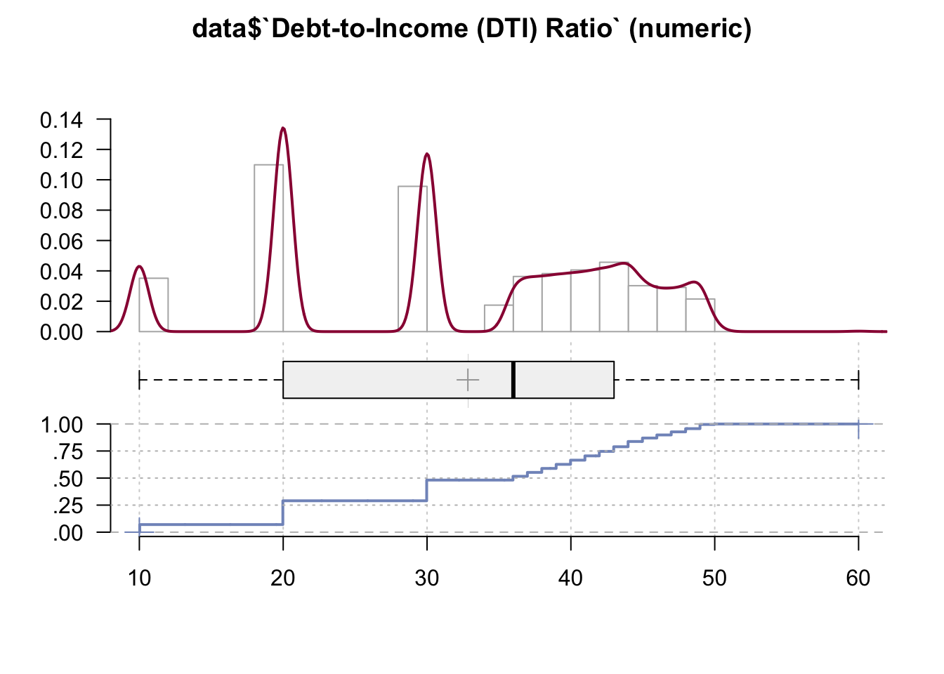
From this graph we may see that many people had 20% and 30% DTI Ratio, which is followed by higher proportions.
The following column does not meet our research questions, so we remove it
data <- data %>% select(-`Discount Points`)Desc(data$`Property Value`)## ----------------------------------------------------------------------------------------------------------------------
## data$`Property Value` (numeric)
##
## length n NAs unique 0s mean meanCI'
## 999'985 999'911 74 368 0 369'372.48 368'934.14
## 100.0% 0.0% 0.0% 369'810.82
##
## .05 .10 .25 median .75 .90 .95
## 125'000.00 155'000.00 225'000.00 325'000.00 465'000.00 635'000.00 765'000.00
##
## range sd vcoef mad IQR skew kurt
## 9'000'000.00 223'638.41 0.61 177'912.00 240'000.00 2.85 26.85
##
## lowest : 5'000.0 (14), 15'000.0 (4), 25'000.0 (90), 35'000.0 (423), 45'000.0 (945)
## highest: 6'405'000.0 (2), 7'005'000.0, 7'105'000.0, 8'305'000.0, 9'005'000.0
##
## ' 95%-CI (classic)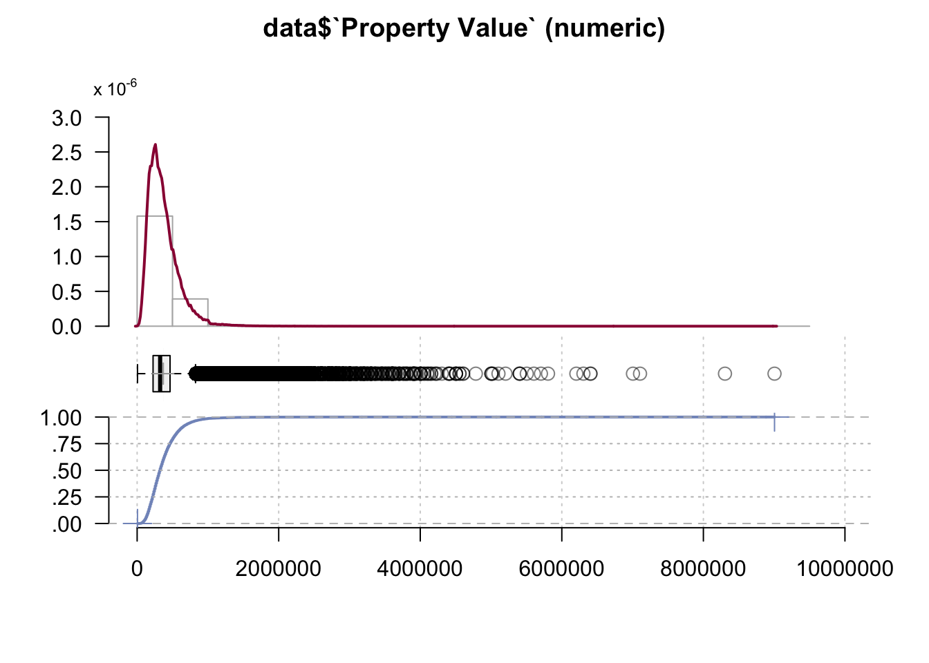
The Property Value is also related to Loan-to-Value Ratio (LTV). 90% of the properties had value of 635 000 but there are several borrowers whose property value is much higher than that.
The next columns should be deleted as they are irrelevant to our research questions
data <- data %>% select(-c("Rural Census Tract", "Lower Mississippi Delta County", "Middle Appalachia County"))Desc(data$`Persistent Poverty County`)## ----------------------------------------------------------------------------------------------------------------------
## data$`Persistent Poverty County` (factor - dichotomous)
##
## length n NAs unique
## 999'985 999'985 0 2
## 100.0% 0.0%
##
## freq perc lci.95 uci.95'
## No 973'872 97.4% 97.4% 97.4%
## Yes 26'113 2.6% 2.6% 2.6%
##
## ' 95%-CI (Wilson)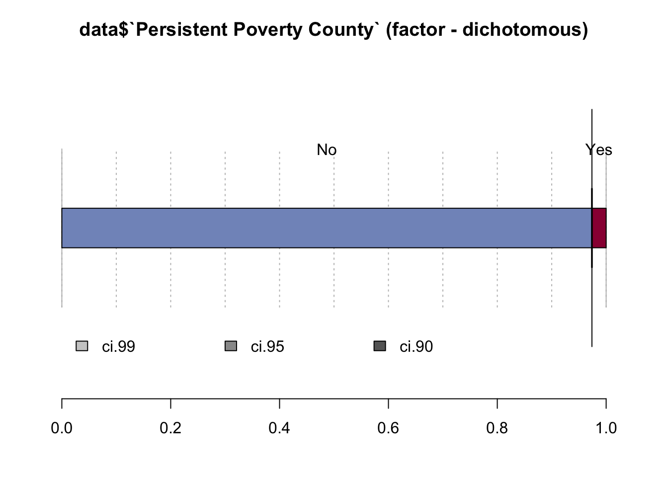
A 2009 U.S. federal law defined a persistent poverty county as one in which “20 percent or more of its population [has lived] in poverty over the past 30 years” according to the Census, which is done every 10 years. Most of the borrowers are not in area of persistent poverty as we can observe from the graph.
Desc(data$`Area of Concentrated Poverty`)## ----------------------------------------------------------------------------------------------------------------------
## data$`Area of Concentrated Poverty` (factor - dichotomous)
##
## length n NAs unique
## 999'985 999'985 0 2
## 100.0% 0.0%
##
## freq perc lci.95 uci.95'
## No 921'216 92.1% 92.1% 92.2%
## Yes 78'769 7.9% 7.8% 7.9%
##
## ' 95%-CI (Wilson)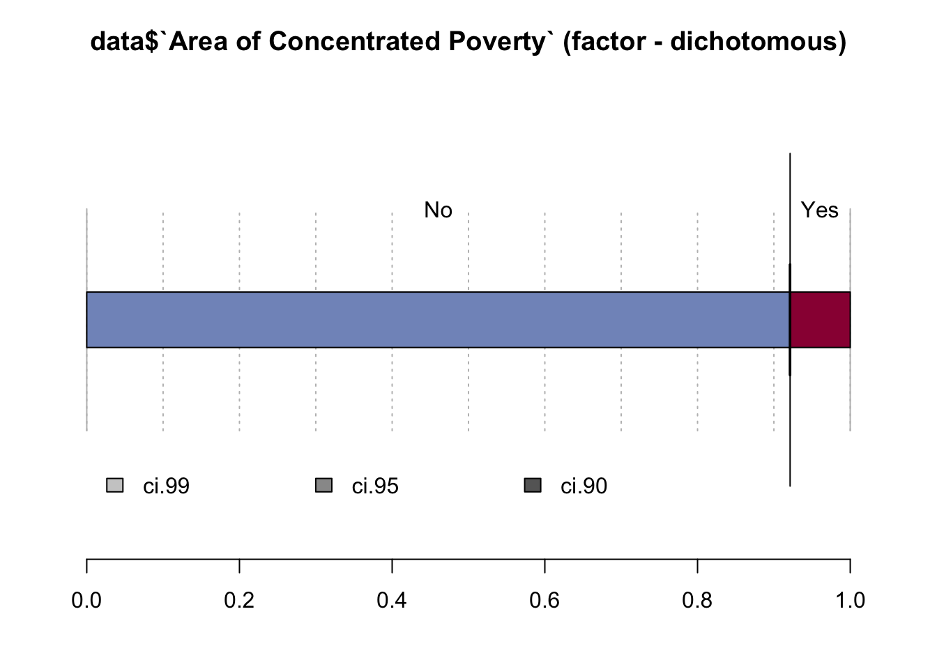
An area of concentrated poverty is defined as a census tract in which more than 40 percent of the households fall below the poverty line. Here we again see that most of the borrowers were not looking for a property in that area.
Based on our findings we need to drop column Persistent Poverty because it correlates with Area of Concentrated Poverty.
data <- data %>% select(-`Persistent Poverty County`)Desc(data$`High Opportunity Area`)## ----------------------------------------------------------------------------------------------------------------------
## data$`High Opportunity Area` (factor - dichotomous)
##
## length n NAs unique
## 999'985 999'985 0 2
## 100.0% 0.0%
##
## freq perc lci.95 uci.95'
## No 811'131 81.1% 81.0% 81.2%
## Yes 188'854 18.9% 18.8% 19.0%
##
## ' 95%-CI (Wilson)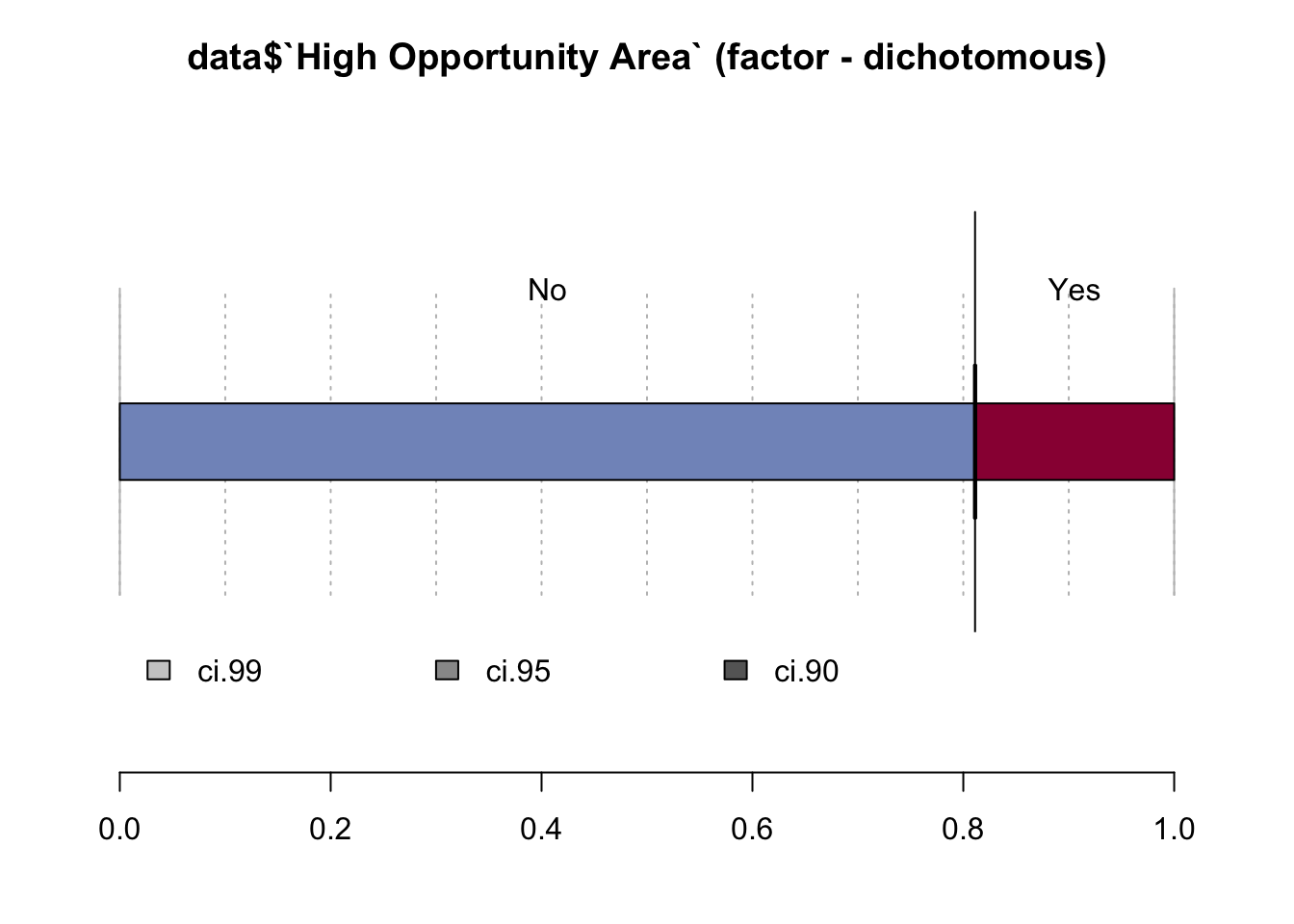
High Opportunity Area generally refers to ares that provide access to certain amenities or community attributes that are believed to increase economic mobility for their residents. High Opportunity Area and Area of Concentrated Poverty should be mutually exclusive as high opportunity area cannot be are of concentrated poverty and vice versa. But we can see that a majority of properties are not labeled as either.
The last column also makes no interest for us so we proceed with deleting it.
data <- data %>% select(-`Qualified Opportunity Zone (QOZ)`)Finally, we have cleaned our data and are now left with the following structure:
summary(data)## Enterprise Flag Local Area Median Income Borrower’s (or Borrowers’) Annual Income Borrower Income Ratio
## Fannie Mae :566099 Min. : 18262 Min. : 0 Min. : 0.000
## Freddie Mac:433886 1st Qu.: 66070 1st Qu.: 65000 1st Qu.: 0.810
## Median : 73783 Median : 96000 Median : 1.200
## Mean : 75430 Mean : 116027 Mean : 1.464
## 3rd Qu.: 81823 3rd Qu.: 141000 3rd Qu.: 1.760
## Max. :133523 Max. :12807000 Max. :218.170
## NA's :848
## Purpose of Loan Number of Borrowers First-Time Home Buyer
## Purchase :544618 Min. :1.000 Yes :232398
## Refinancing :242591 1st Qu.:1.000 No :767322
## Home improvement : 535 Median :1.000 NA's: 265
## Refinancing cash-out:212241 Mean :1.471
## 3rd Qu.:2.000
## Max. :6.000
##
## Borrower Race Co-Borrower Race Borrower Gender
## American Indian or Alaska Native : 4341 American Indian or Alaska Native : 2105 Male :612829
## Asian : 70216 Asian : 30770 Female:307547
## Black or African American : 39137 Black or African American : 11001 NA's : 79609
## Native Hawaiian or Other Pacific Islander: 2439 Native Hawaiian or Other Pacific Islander: 1245
## White :742115 White :352092
## NA's :141737 no co-borrower : 0
## NA's :602772
## Co-Borrower Gender Age of Borrower Age of Co-Borrower
## Male :107228 35 to 44 years old:257033 35 to 44 years old:115052
## Female:317215 25 to 34 years old:231205 25 to 34 years old:109971
## NA's :575542 45 to 54 years old:211435 45 to 54 years old: 93271
## 55 to 64 years old:164166 55 to 64 years old: 80302
## 65 to 74 years old: 85732 65 to 74 years old: 44432
## (Other) : 50389 (Other) : 21659
## NA's : 25 NA's :535298
## Occupancy Code Property Type
## Principal Residence/Owner-Occupied property:897838 one to four-family (other than manufactured housing):993218
## Second Home : 40679 manufactured housing : 6767
## Investment property : 61468
##
##
##
##
## Loan-to-Value Ratio (LTV) Date of Mortgage Note Term of Mortgage at Origination
## Min. : 3.23 Originated in same calendar year as acquired :900004 Min. : 60.0
## 1st Qu.: 67.34 Originated prior to calendar year of acquisition: 99981 1st Qu.:360.0
## Median : 80.00 Median :360.0
## Mean : 75.62 Mean :332.5
## 3rd Qu.: 90.00 3rd Qu.:360.0
## Max. :308.00 Max. :480.0
## NA's :3
## Number of Units Interest Rate at Origination Note Amount Debt-to-Income (DTI) Ratio Property Value
## Min. :1.000 Min. :0.62 Min. : 5000 Min. :10.00 Min. : 5000
## 1st Qu.:1.000 1st Qu.:3.87 1st Qu.: 155000 1st Qu.:20.00 1st Qu.: 225000
## Median :1.000 Median :4.12 Median : 235000 Median :36.00 Median : 325000
## Mean :1.025 Mean :4.24 Mean : 260106 Mean :32.84 Mean : 369372
## 3rd Qu.:1.000 3rd Qu.:4.62 3rd Qu.: 345000 3rd Qu.:43.00 3rd Qu.: 465000
## Max. :4.000 Max. :8.55 Max. :1395000 Max. :60.00 Max. :9005000
## NA's :74 NA's :74 NA's :84 NA's :74
## Area of Concentrated Poverty High Opportunity Area
## No :921216 No :811131
## Yes: 78769 Yes:188854
##
##
##
##
##