4 Decluttering
4.1 Decluttering rows
Next, we use the technique of decluttering to reduce the number of overall rows. We can only delete the rows which have no value for us. That means rows that either have no information for us because of only missing values or they are not relevant for our research question. In the first case, we can proceed by identifying the percentage of entries per row, which are actually NA. Afterwards, we plot these number to check how much data per row is missing and whether there are some extreme cases where a lot of data is missing.
na_rows <- apply(is.na(data),1,sum)/ncol(data)
options(scipen=999)
plot(na_rows, type="h", xlab = "Index", ylab = "NA Frequency")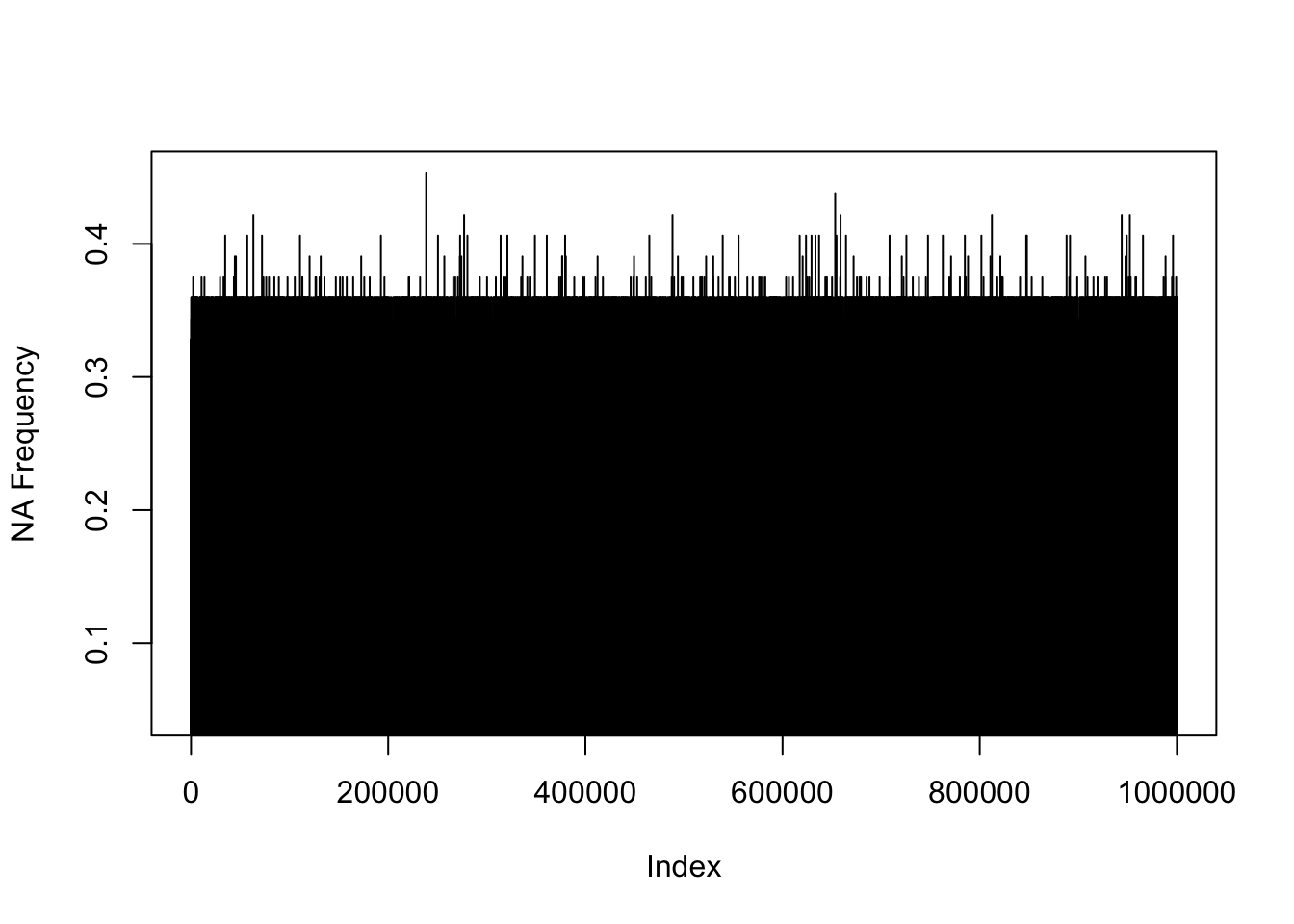
From the chart above we can conclude that the severity of NA values is not huge, however, there seem to be a number of entries which miss more data than the majority of records. But overall, we have no records to delete. There are also no rows that are currently ‘not relevant’ so we can proceed to the decluttering columns step.
4.2 Decluttering columns
For decluttering the columns we will use again the same two criteria as previously mentioned. That means we are going to eliminate all columns with (almost) all entries missing and we are going to delete columns which only have one unique value.
Following the standard procedure, we create a table to help us with an overview of the missingness and uniqueness of values in our columns. First, we calculate the percentage of missing values per column.
missing_vals <- as.matrix(data %>% is.na %>% colSums)
missing_vals_rel <- round(100*missing_vals/nrow(data),2)
Then, we to do the same for the unique values in the columns:
unique_vals <- t(as.matrix(data %>% summarise_all(n_distinct)))
unique_vals_rel <-  round(100*unique_vals/nrow(data),2)
Last but not least, we can summarize the findings in a small data summary table:
data_summary <- data.frame(missing_vals, missing_vals_rel, unique_vals, unique_vals_rel)
colnames(data_summary) <- c("NAs", "NAs_rel", "Unique", "Unique_rel")
data_summary
## NAs NAs_rel Unique Unique_rel
## Enterprise Flag 0 0.00 2 0.00
## Record Number 0 0.00 1000000 100.00
## US Postal State Code 0 0.00 54 0.01
## Metropolitan Statistical Area (MSA) Code 0 0.00 393 0.04
## County - 2010 Census 0 0.00 317 0.03
## Census Tract - 2010 Census 159 0.02 23161 2.32
## 2010 Census Tract - Percent Minority 423 0.04 9712 0.97
## 2010 Census Tract - Median Income 848 0.08 37191 3.72
## Local Area Median Income 848 0.08 1222 0.12
## Tract Income Ratio 848 0.08 346 0.03
## Borrower’s (or Borrowers’) Annual Income 0 0.00 1619 0.16
## Area Median Family Income (2019) 1 0.00 422 0.04
## Borrower Income Ratio 15 0.00 1984 0.20
## Acquisition Unpaid Principal Balance (UPB) 0 0.00 131 0.01
## Purpose of Loan 0 0.00 4 0.00
## Federal Guarantee 0 0.00 4 0.00
## Number of Borrowers 0 0.00 6 0.00
## First-Time Home Buyer 265 0.03 3 0.00
## Borrower Race1 141739 14.17 6 0.00
## Borrower Race2 986242 98.62 6 0.00
## Borrower Race3 999528 99.95 6 0.00
## Borrower Race4 999948 99.99 5 0.00
## Borrower Race5 999986 100.00 3 0.00
## Borrower Ethnicity 143473 14.35 3 0.00
## Co-Borrower Race1 602783 60.28 6 0.00
## Co-Borrower Race2 990779 99.08 6 0.00
## Co-Borrower Race3 999763 99.98 6 0.00
## Co-Borrower Race4 999977 100.00 5 0.00
## Co-Borrower Race5 999997 100.00 3 0.00
## Co-Borrower Ethnicity 609922 60.99 3 0.00
## Borrower Gender 79610 7.96 3 0.00
## Co-Borrower Gender 575553 57.56 3 0.00
## Age of Borrower 25 0.00 8 0.00
## Age of Co-Borrower 535309 53.53 8 0.00
## Occupancy Code 0 0.00 3 0.00
## Rate Spread 963661 96.37 298 0.03
## HOEPA Status 0 0.00 1 0.00
## Property Type 0 0.00 2 0.00
## Lien Status 0 0.00 1 0.00
## Borrower Age 62 or older 25 0.00 3 0.00
## Co-Borrower Age 62 or older 535309 53.53 3 0.00
## Loan-to-Value Ratio (LTV) 3 0.00 9168 0.92
## Date of Mortgage Note 0 0.00 2 0.00
## Term of Mortgage at Origination 0 0.00 156 0.02
## Number of Units 0 0.00 4 0.00
## Interest Rate at Origination 74 0.01 367 0.04
## Note Amount 74 0.01 131 0.01
## Preapproval 679221 67.92 3 0.00
## Application Channel 204345 20.43 4 0.00
## Automated Underwriting System (AUS) 11919 1.19 4 0.00
## Credit Score Model - Borrower 216866 21.69 4 0.00
## Credit Score Model - Co-Borrower 217164 21.72 5 0.00
## Debt-to-Income (DTI) Ratio 97 0.01 20 0.00
## Discount Points 294369 29.44 140862 14.09
## Introductory Rate Period 992288 99.23 11 0.00
## Manufactured Home – Land Property Interest 997977 99.80 4 0.00
## Property Value 74 0.01 369 0.04
## Rural Census Tract 0 0.00 2 0.00
## Lower Mississippi Delta County 0 0.00 2 0.00
## Middle Appalachia County 0 0.00 2 0.00
## Persistent Poverty County 0 0.00 2 0.00
## Area of Concentrated Poverty 0 0.00 2 0.00
## High Opportunity Area 0 0.00 2 0.00
## Qualified Opportunity Zone (QOZ) 0 0.00 2 0.00Based on the table, we can see that there are some columns exhibiting 100 percent missing values or having only one unique value, such as Borrower Race5, HOEPA Status, or Introductory Rate Period. We delete these columns from our data as there is no relevant information to be gained. Furthermore, we also delete columns that have an extremely high proportion of missing values of more than 96% as these columns would not be useful either.
uniques <- rownames(data_summary)[which(data_summary$Unique==1)]
full_NA <- rownames(data_summary)[which(data_summary$NAs_rel==100)]
high_NA <- rownames(data_summary)[which(data_summary$NAs_rel>96&data_summary$NAs_rel<100)]

col_del_ind <- match(unique(c(uniques,full_NA,high_NA)),colnames(data)) # unique, because we can have some double counts
data <- data[,-col_del_ind]

dim(data)
## [1] 1000000 51Looking at the table above, we see that we have managed to drop 13 unnecessary columns, leaving us with remaining 51 columns that need to be further qualitatively assessed.