2 Into the Tidyverse
What do we mean by this tidyverse thing?
The tidyverse is an opinionated collection of R packages designed for data science. All packages share an underlying design philosophy, grammar, and data structures. [Source]
We are going to look at two packages in particular. dplyr will let us manipulate and summarize our data. We’ll cover this now. ggplot2 lets us graph our data and is covered in Section 3.
We’ll open up a new R script and work with the NC Breweries data again. Make sure that you are in the project file for this course. You should see elon-r-datacamp in the upper right project dropdown menu in RStudio.
Our goal: Get the data organized in a way that lets us do our analysis.
2.1 Getting Our Data
Open up a blank R script and bring in the tidyverse and here. Then, load in the breweries data. I’ve given you two options for loading in data. The first assumes that the file is in a folder called data, one level down from your project folder. The second goes and gets the data directly from my Github page. I’ve commented that way out, but you can use this method!
# install.package("tidyverse")
library(tidyverse)
library(here)
ncbreweries <- read_csv(here::here("data", "ncbreweries.csv"))
# ncbreweries <- read_csv("https://raw.githubusercontent.com/aaiken1/elon-r-datacamp/main/data/ncbreweries.csv")
If you are familiar with pivot tables in Excel, a lot of what we’re about to do is the “code” for slicing and dicing your data in a similar fashion. The end goal is often to get our data set up for some type of statistical analysis, creating a plot, etc.
Let’s check and see what R thinks this brewery data is. A class in R is bascially the type of thing something is. You can read more here at Datacamp. This gets into object oriented programming, or OOP and is beyond the scope of what we’re doing here. However, you’ll need to at least be familiar with these ideas to get the full benefit of using something like R.
class(ncbreweries)
#> [1] "spec_tbl_df" "tbl_df"      "tbl"         "data.frame"
We’ve read in the data using the read_csv function, which comes with the readr package and is included as part of the tidyverse universe. R thinks that this data file is a special kind of data frame, called a tbl or tibble.
OK, but what is a data frame? And tibble sounds funny. We need to talk about data.
2.2 tidy Data
You might be familiar with data when in something like an Excel file. You have rows and columns. What defines nice and neat, or tidy data?
The characteristics of tidy data are:
- Each variable forms a column.
- Each observation forms a row.
- Each type of observational unit forms a table.
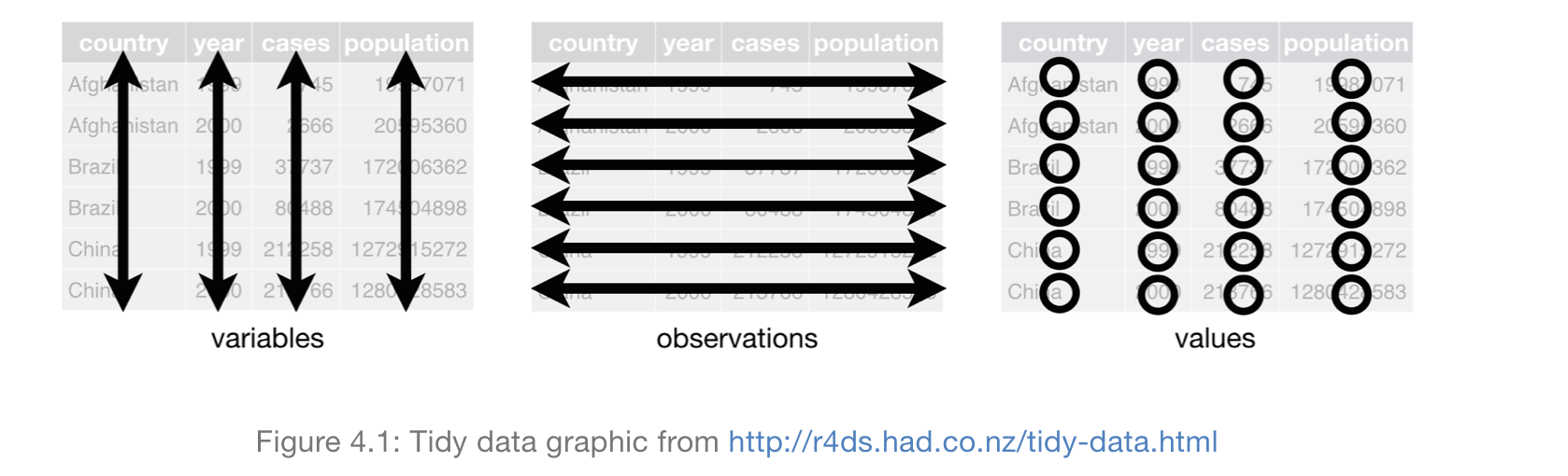
Figure 2.1: What do we mean by tidy data?
The tidyverse is a series of packages that work well together and will help you get your data “tidy”.
OK, but what are tibbles? Think of a data frame (or, data.frame to R) as an Excel file with the first row as the names of the variables and then each row underneath that as an observation. tibbles are just special data frames. They are “spreadsheets”, a place to keep our data.
Type vignette("tibble") in the Console to see more, or go to the Help panel and search for “tibble”.
2.2.1 tidyverse vs. Base R
I should note that there is a “tidyverse vs. base R” debate. Base R doesn’t include the tidyverse and sticks to functions, methods, and classes that come with the R you install without any packages.
Many R users think that you should learn the tidyverse first. I agree. Why?
- The
tidyversedocumentation and community support are outstanding. Folks are friendly! - Having a consistent philosophy and syntax makes it much easier to learn.
- For data cleaning, wrangling and plotting… the tidyverse is really a no-brainer.
One point of convenience is that there is often a direct correspondence between a tidyverse command and its base R equivalent.
These invariably follow a tidyverse::snake_case vs base::period.case rule. For example,
-
?readr::read_csvvs.?utils::read.csv -
?tibble::data_framevs.?base::data.frame -
?dplyr::if_elsevs.?base::ifelse
If you call up the above examples, you’ll see that the tidyverse alternative typically offers some enhancements or other useful options (and sometimes restrictions) over its base counterpart. If you see an underscore, _, in a function, then you’re in the tidyverse.
There are always many ways to achieve a single goal in R. So, when you start searching for solutions to your coding problems, just keep that in mind.
2.2.2 Pipes: Step by Step
Figure 2.2: This is not a pipe.
You can think about the following sequence of actions - find key, unlock car, start car, drive to school, park.
Expressed as a set of nested functions in R pseudocode, this would look like… a mess:
park(drive(start_car(find("keys")), to = "campus"))Writing it out using pipes give it a more natural (and easier to read) structure:
The pipe operator is denoted %>% and is automatically loaded with the tidyverse, as part of the magrittr package. Get it?
Pipes dramatically improve the experience of reading and writing code. Here’s another example:
## These next two lines of code do exactly the same thing.
mpg %>% filter(manufacturer=="audi") %>% group_by(model) %>% summarize(hwy_mean = mean(hwy))

summarize(group_by(filter(mpg, manufacturer=="audi"), model), hwy_mean = mean(hwy))
The first line reads from left to right, exactly how I thought of the operations in my head. - Take this data set (mpg), do this (filter), then do this (group by), then summarize some variable (hwy).
The second line totally inverts this logical order, as the final operation comes first! Who wants to read things inside out?
The piped version of the code is even more readable if we write it over several lines. Here it is again and, this time, I’ll run it for good measure so you can see the output:
mpg %>%
  filter(manufacturer=="audi") %>%
  group_by(model) %>%
  summarize(hwy_mean = mean(hwy))
#> # A tibble: 3 × 2
#>   model      hwy_mean
#>   <chr>         <dbl>
#> 1 a4             28.3
#> 2 a4 quattro     25.8
#> 3 a6 quattro     24
Remember: Using vertical space costs nothing and makes for much more readable/writeable code than cramming things horizontally.
To send results to a function argument other than first one or to use the previous result for multiple arguments, use .:
starwars %>%
  filter(species == "Human") %>%
  lm(mass ~ height, data = .)
#>
#> Call:
#> lm(formula = mass ~ height, data = .)
#>
#> Coefficients:
#> (Intercept)       height
#>     -116.58         1.11
I just ran a regression using the starswars data that comes built-in to the tidyverse package. Turns out taller characters weigh more. Makes sense. This code is taking the starwars tibble, keeping just the humans, and then running a simple linear regression that uses height to explain mass.
You can see the first few rows of any data set using the head function. There’s also a similar tail option.
head(starwars)
#> # A tibble: 6 × 14
#> name height mass hair_…¹ skin_…² eye_c…³ birth…⁴ sex
#> <chr> <int> <dbl> <chr> <chr> <chr> <dbl> <chr>
#> 1 Luke S… 172 77 blond fair blue 19 male
#> 2 C-3PO 167 75 <NA> gold yellow 112 none
#> 3 R2-D2 96 32 <NA> white,… red 33 none
#> 4 Darth … 202 136 none white yellow 41.9 male
#> 5 Leia O… 150 49 brown light brown 19 fema…
#> 6 Owen L… 178 120 brown,… light blue 52 male
#> # … with 6 more variables: gender <chr>, homeworld <chr>,
#> # species <chr>, films <list>, vehicles <list>,
#> # starships <list>, and abbreviated variable names
#> # ¹hair_color, ²skin_color, ³eye_color, ⁴birth_yearBy the way, there are now pipes in Base R.
2.3 dplyr
OK, let’s get back to our breweries data that we should now have in our Global Environment. You can view the names of variables in a data frame/tibble via the names function. We can also use glimpse, which will also tell us the number of rows, columns, and variable types.
We haven’t talked about variable types yet. For our purposes, there are characters (
There are many ways to peak at our data. You can double click on the data in the Global Environment to see the whole thing like a spreadsheet. This is the same as the view function.
names(ncbreweries)
#> [1] "name"      "city"      "type"      "beercount"
#> [5] "est"       "status"    "url"
glimpse(ncbreweries)
#> Rows: 251
#> Columns: 7
#> $ name      <chr> "217 Brew Works", "3rd Rock Brewing Comp…
#> $ city      <chr> "Wilson", "Trenton", "Cherokee", "Andrew…
#> $ type      <chr> "Microbrewery", "Microbrewery", "Client …
#> $ beercount <dbl> 10, 12, 1, 18, 8, 78, 15, 87, 106, 59, 1…
#> $ est       <dbl> 2017, 2016, 2018, 2014, 2017, 2013, 2017…
#> $ status    <chr> "Active", "Active", "Active", "Active", …
#> $ url       <chr> "https://www.ratebeer.com//brewers/217-b…
We are now going to take this data set and look at some of the dplyr functions.
-
filter: pick rows matching criteria -
slice: pick rows using index(es) -
select: pick columns by name -
pull: grab a column as a vector -
arrange: reorder rows -
mutate: add new variables -
distinct: filter for unique rows -
sample_n/sample_frac: randomly sample rows -
summarize: reduce variables to values - … (many more)
Because all of these functions come from the dplyr package, then they all follow similar rules.
- First argument is always a data frame, or tibble.
- Subsequent arguments say what to do with that data frame
- Always return a data frame
- This won’t change the original data frame unless you tell it to.
Remember, the %>% operator in dplyr functions is called the pipe operator. This means you “pipe” the output of the previous line of code as the first input of the next line of code.
I am not saving any of this to memory. So, when we filter, get rid of missings, etc., we will see the output below. But, we are not changing the original data, or saving the data to a new file, unless we do an extra sep
We would use the assignment operator <-. For example, new_data <- our code.
You can find more examples and syntax in Chapter 5 of R for Data Science.
2.3.1 filter
Let’s find breweries in Durham County. To do that, we’ll use dplyr::filter.
ncbreweries %>%
dplyr::filter(city == "Durham")
#> # A tibble: 9 × 7
#> name city type beerc…¹ est status url
#> <chr> <chr> <chr> <dbl> <dbl> <chr> <chr>
#> 1 Barrel Culture Bre… Durh… Micr… 29 2017 Active http…
#> 2 Bull City Burger a… Durh… Brew… 64 2011 Active http…
#> 3 Bull City Ciderwor… Durh… Comm… 9 2014 Active http…
#> 4 Bull Durham Beer C… Durh… Micr… 7 2015 Active http…
#> 5 Durty Bull Brewing… Durh… Micr… 19 2016 Active http…
#> 6 Fullsteam Brewery Durh… Micr… 131 2009 Active http…
#> 7 Ponysaurus Brewing… Durh… Micr… 26 2013 Active http…
#> 8 G2B Gastropub & Br… Durh… Brew… 18 2015 Closed http…
#> 9 Triangle Brewing C… Durh… Micr… 21 2007 Closed http…
#> # … with abbreviated variable name ¹beercountThe :: tells R where to look for the filter function. It lives in dplyr. You don’t actually need that, though things can go wrong without it, if there are two identically named functions from different packages! Because we loaded tidyverse and, therefore, dplyr, last, it will mask other functions of the same name. In other words, when we type filter, R is going to assume that we want the one from dplyr.
And, because we are using a %>%, we start with the data frame. The data frame then gets passed on through. So, you don’t need to specifiy a data frame to filter. It knows that we want to use ncbreweries.
Here’s dplyr::filter for many conditions. Other conditions that you could use include >, <, >=, <=, and != for not equal. Note that equal is == and not =.
Let’s find breweries in Durham that were founded in 2014.
ncbreweries %>%
filter(city == "Durham", est == 2014)
#> # A tibble: 1 × 7
#> name city type beerc…¹ est status url
#> <chr> <chr> <chr> <dbl> <dbl> <chr> <chr>
#> 1 Bull City Ciderwor… Durh… Comm… 9 2014 Active http…
#> # … with abbreviated variable name ¹beercountLooks like there was just one.
A very common filter() use case is identifying (or removing) observations with missing data. is.na returns a logical vector (i.e. a bunch of TRUE and FALSE values) that will be TRUE if a value of the column referenced is missing/not available.
ncbreweries %>%
  filter(is.na(city))
#> # A tibble: 0 × 7
#> # … with 7 variables: name <chr>, city <chr>, type <chr>,
#> #   beercount <dbl>, est <dbl>, status <chr>, url <chr>
To remove missing observations, simply use negation: filter(!is.na(city)). This data set doesn’t have any missing city values.
You can also use dplyr with regex (or Regular Expressions). regex is just a series of commands to deal with strings/text/characters. Here’s one basic example. filter is looking for a True/False from the arguments inside. grepl returns True if the name column contains the string “Bear” anywhere in it. So, you’ll get a data frame (tibble) that only has breweries with “Bear” in their name.
ncbreweries %>%
filter(grepl("Bear", name))
#> # A tibble: 2 × 7
#> name city type beerc…¹ est status url
#> <chr> <chr> <chr> <dbl> <dbl> <chr> <chr>
#> 1 Bear Creek Brews Bear… Micr… 6 2012 Active http…
#> 2 BearWaters Brewing… Cant… Micr… 39 2012 Active http…
#> # … with abbreviated variable name ¹beercount2.3.2 select
You can use dplyr::select to keep just the variables that you want.
ncbreweries %>%
  filter(city == "Durham", beercount > 10) %>%
  select(name, type)
#> # A tibble: 7 × 2
#>   name                                type
#>   <chr>                               <chr>
#> 1 Barrel Culture Brewing and Blending Microbrewery
#> 2 Bull City Burger and Brewery        Brewpub/Brewery
#> 3 Durty Bull Brewing Company          Microbrewery
#> 4 Fullsteam Brewery                   Microbrewery
#> 5 Ponysaurus Brewing Co.              Microbrewery
#> 6 G2B Gastropub & Brewery             Brewpub/Brewery
#> 7 Triangle Brewing Company            Microbrewery
You can also exclude variables. The - means “select everything but”.
ncbreweries %>%
select(-type)
#> # A tibble: 251 × 6
#> name city beerc…¹ est status url
#> <chr> <chr> <dbl> <dbl> <chr> <chr>
#> 1 217 Brew Works Wils… 10 2017 Active http…
#> 2 3rd Rock Brewing Company Tren… 12 2016 Active http…
#> 3 7 Clans Brewing Cher… 1 2018 Active http…
#> 4 Andrews Brewing Company Andr… 18 2014 Active http…
#> 5 Angry Troll Brewing Elkin 8 2017 Active http…
#> 6 Appalachian Mountain Br… Boone 78 2013 Active http…
#> 7 Archetype Brewing Ashe… 15 2017 Active http…
#> 8 Asheville Brewing Compa… Ashe… 87 2003 Active http…
#> 9 Ass Clown Brewing Compa… Corn… 106 2011 Active http…
#> 10 Aviator Brewing Company Fuqu… 59 2008 Active http…
#> # … with 241 more rows, and abbreviated variable name
#> # ¹beercountSometimes you have hundreds of variables and you don’t want to type them all out. You can use “first:last” for consecutive columns, or just list out the columns separated by commas.
ncbreweries %>%
  select(city:beercount)
#> # A tibble: 251 × 3
#>    city          type          beercount
#>    <chr>         <chr>             <dbl>
#>  1 Wilson        Microbrewery         10
#>  2 Trenton       Microbrewery         12
#>  3 Cherokee      Client Brewer         1
#>  4 Andrews       Microbrewery         18
#>  5 Elkin         Microbrewery          8
#>  6 Boone         Microbrewery         78
#>  7 Asheville     Microbrewery         15
#>  8 Asheville     Brewpub              87
#>  9 Cornelius     Microbrewery        106
#> 10 Fuquay Varina Microbrewery         59
#> # … with 241 more rows
You can use dplyr::select to rename columns, or variables. The new name goes first.
ncbreweries %>%
  select(town=city)
#> # A tibble: 251 × 1
#>    town
#>    <chr>
#>  1 Wilson
#>  2 Trenton
#>  3 Cherokee
#>  4 Andrews
#>  5 Elkin
#>  6 Boone
#>  7 Asheville
#>  8 Asheville
#>  9 Cornelius
#> 10 Fuquay Varina
#> # … with 241 more rows
The select(contains(PATTERN)) option provides a nice shortcut in relevant cases and gives us another example of using text. Only one variable contains “type” in this case.
ncbreweries %>%
  select(name, contains("type"))
#> # A tibble: 251 × 2
#>    name                         type
#>    <chr>                        <chr>
#>  1 217 Brew Works               Microbrewery
#>  2 3rd Rock Brewing Company     Microbrewery
#>  3 7 Clans Brewing              Client Brewer
#>  4 Andrews Brewing Company      Microbrewery
#>  5 Angry Troll Brewing          Microbrewery
#>  6 Appalachian Mountain Brewery Microbrewery
#>  7 Archetype Brewing            Microbrewery
#>  8 Asheville Brewing Company    Brewpub
#>  9 Ass Clown Brewing Company    Microbrewery
#> 10 Aviator Brewing Company      Microbrewery
#> # … with 241 more rows
The select(..., everything()) option is another useful shortcut if you only want to bring some variable(s) to the “front” of a data frame.
ncbreweries %>%
select(name, beercount, everything())
#> # A tibble: 251 × 7
#> name beerc…¹ city type est status url
#> <chr> <dbl> <chr> <chr> <dbl> <chr> <chr>
#> 1 217 Brew Works 10 Wils… Micr… 2017 Active http…
#> 2 3rd Rock Brewing … 12 Tren… Micr… 2016 Active http…
#> 3 7 Clans Brewing 1 Cher… Clie… 2018 Active http…
#> 4 Andrews Brewing C… 18 Andr… Micr… 2014 Active http…
#> 5 Angry Troll Brewi… 8 Elkin Micr… 2017 Active http…
#> 6 Appalachian Mount… 78 Boone Micr… 2013 Active http…
#> 7 Archetype Brewing 15 Ashe… Micr… 2017 Active http…
#> 8 Asheville Brewing… 87 Ashe… Brew… 2003 Active http…
#> 9 Ass Clown Brewing… 106 Corn… Micr… 2011 Active http…
#> 10 Aviator Brewing C… 59 Fuqu… Micr… 2008 Active http…
#> # … with 241 more rows, and abbreviated variable name
#> # ¹beercount2.3.3 slicing
You use dplyr::slice to keep certain row numbers, or observations.
Here are the first five observations of the data frame/tibble. This is a lot like the Base R head() function.
ncbreweries %>%
slice(1:5)
#> # A tibble: 5 × 7
#> name city type beerc…¹ est status url
#> <chr> <chr> <chr> <dbl> <dbl> <chr> <chr>
#> 1 217 Brew Works Wils… Micr… 10 2017 Active http…
#> 2 3rd Rock Brewing C… Tren… Micr… 12 2016 Active http…
#> 3 7 Clans Brewing Cher… Clie… 1 2018 Active http…
#> 4 Andrews Brewing Co… Andr… Micr… 18 2014 Active http…
#> 5 Angry Troll Brewing Elkin Micr… 8 2017 Active http…
#> # … with abbreviated variable name ¹beercountYou can also grab the last five observations of the tibble. Notice the use of nrow, a Base R function. I am finding the number of rows in this data frame and then saving that to the variable last_row. Check out the Global Environment.
last_row <- nrow(ncbreweries)
ncbreweries %>%
slice((last_row - 4):last_row)
#> # A tibble: 5 × 7
#> name city type beerc…¹ est status url
#> <chr> <chr> <chr> <dbl> <dbl> <chr> <chr>
#> 1 Sweet Taters Rock… Brew… 9 2016 Closed http…
#> 2 Triangle Brewing C… Durh… Micr… 21 2007 Closed http…
#> 3 White Rabbit Brewi… Angi… Micr… 19 2013 Closed http…
#> 4 Williamsville Brew… Farm… Brew… 5 2000 Closed http…
#> 5 Wolf Beer Company Wilm… Clie… 2 2009 Closed http…
#> # … with abbreviated variable name ¹beercount2.3.4 sampling
We can also choose a random sample from our data set. Notice that I am now saving, or assigning the resulting data to a new data frame/tibble. I then use the dim function to get the dimensions (rows and columns) of the new data.
sample_n: randomly sample 5 observations
sample_frac: randomly sample 20% of observations
ncbreweries_perc20 <-ncbreweries %>%
  sample_frac(0.2, replace = FALSE)
dim(ncbreweries_perc20)
#> [1] 50  7
2.3.5 distinct
Sometimes you have duplicate values that you want to get rid of. For example, suppose we just wanted to see the distinct values for city and brewery type in our data? We can use dplyr::distinct to filter for unique rows
We can then use arrange to sort our columns. Character columns get sorted alphabetically. We can also arrange items in descending order using arrange(desc()).
ncbreweries %>%
  select(city, type) %>%
  distinct() %>%
  arrange(type, city)
#> # A tibble: 138 × 2
#>    city          type
#>    <chr>         <chr>
#>  1 Andrews       Brewpub
#>  2 Arden         Brewpub
#>  3 Asheville     Brewpub
#>  4 Boone         Brewpub
#>  5 Chapel Hill   Brewpub
#>  6 Charlotte     Brewpub
#>  7 Farmville     Brewpub
#>  8 Fayetteville  Brewpub
#>  9 Fuqauy Varina Brewpub
#> 10 Greenville    Brewpub
#> # … with 128 more rows
There are 138 city x type pairs in our data.
2.3.6 summarize
dplyr::summarize let’s us calculate things like means, medians, standard deviations, etc. This will create a new data frame. Here’s an example that looks across all of the breweries and calculates the mean number of beers, the standard deviation, and the number of breweries included.
ncbreweries %>%
  summarize(avg_beercount = mean(beercount), stddev_beercount = sd(beercount), n_beercount = n())
#> # A tibble: 1 × 3
#>   avg_beercount stddev_beercount n_beercount
#>           <dbl>            <dbl>       <int>
#> 1          33.0             43.7         251
You can do calculations by group using ddplyr::group_by. This is very common and basically like creating pivot tables in Excel. The group_by goes first, then the summarize. Use ungroup() after performing the work in the groups to prevent mistakes later on. If you don’t include it, R will still look at this data frame as grouped.
ncbreweries %>%
  group_by(type) %>%
  summarize(avg_beercount = mean(beercount)) %>%
  ungroup()
#> # A tibble: 5 × 2
#>   type               avg_beercount
#>   <chr>                      <dbl>
#> 1 Brewpub                     44.9
#> 2 Brewpub/Brewery             37.7
#> 3 Client Brewer                5
#> 4 Commercial Brewery          10.7
#> 5 Microbrewery                31.3
Including “na.rm = T” is usually a good idea with summarize functions. Otherwise, any missing value will propogate to the summarized value too. You’ll get just a single NA value. Let’s go back to the starwars for just a second, as it has some missing data.
## Probably not what we want
starwars %>%
  summarize(mean_height = mean(height))
#> # A tibble: 1 × 1
#>   mean_height
#>         <dbl>
#> 1          NA
## Much better
starwars %>%
  summarize(mean_height = mean(height, na.rm = T))
#> # A tibble: 1 × 1
#>   mean_height
#>         <dbl>
#> 1        174.
OK, that makes more sense!
2.3.7 count
We can also simply count by groups using dplyr::count.
ncbreweries %>%
  count(type)
#> # A tibble: 5 × 2
#>   type                   n
#>   <chr>              <int>
#> 1 Brewpub               33
#> 2 Brewpub/Brewery       41
#> 3 Client Brewer          9
#> 4 Commercial Brewery     3
#> 5 Microbrewery         165
You can also count pairs, or other combinations.
ncbreweries %>%
  count(city, type)
#> # A tibble: 138 × 3
#>    city      type                n
#>    <chr>     <chr>           <int>
#>  1 Aberdeen  Microbrewery        1
#>  2 Andrews   Brewpub             1
#>  3 Andrews   Microbrewery        2
#>  4 Angier    Microbrewery        2
#>  5 Apex      Brewpub/Brewery     1
#>  6 Apex      Microbrewery        2
#>  7 Arden     Brewpub             1
#>  8 Asheboro  Microbrewery        1
#>  9 Asheville Brewpub             5
#> 10 Asheville Brewpub/Brewery     5
#> # … with 128 more rows
2.3.8 mutate
Let’s actually create some new variables. We’ll use dplyr::mutate to do this.
You will usually be creating a new variable from existing data. mutate() is order aware, so you can chain multiple mutates in a single call. In other words, you can create a new variable and then use it to create the next variable.
There’s also transmute(), which will replace the variable being used. mutate() adds a new variable, but doesn’t drop anything.
Let’s combine mutate with case_when to create a new variable called est_category that is set to either “old” or “new”. We’ll then create counts by that new category.
ncbreweries %>%
  mutate(est_category = case_when(
    est < 2000       ~ "old",
    est >= 2000     ~ "new"
  )) %>%
  count(est_category)
#> # A tibble: 2 × 2
#>   est_category     n
#>   <chr>        <int>
#> 1 new            241
#> 2 old             10
When we’re creating new variables, things can get a bit complicated. There are many ways to do the same thing sometimes. Different methods create different types of variables. Here, the logical variable new is TRUE if the brewery was founded in 2000 or later. The character variable est_category is either “New” or “Old”. Both tell you the same thing.
To do this, we are using two mutate functions. One for each new variable.
ncbreweries %>%
mutate(new = est >= 2000) %>%
mutate(est_category = ifelse(est >= 2000, "new", "old"))
#> # A tibble: 251 × 9
#> name city type beerc…¹ est status url new
#> <chr> <chr> <chr> <dbl> <dbl> <chr> <chr> <lgl>
#> 1 217 Brew Wo… Wils… Micr… 10 2017 Active http… TRUE
#> 2 3rd Rock Br… Tren… Micr… 12 2016 Active http… TRUE
#> 3 7 Clans Bre… Cher… Clie… 1 2018 Active http… TRUE
#> 4 Andrews Bre… Andr… Micr… 18 2014 Active http… TRUE
#> 5 Angry Troll… Elkin Micr… 8 2017 Active http… TRUE
#> 6 Appalachian… Boone Micr… 78 2013 Active http… TRUE
#> 7 Archetype B… Ashe… Micr… 15 2017 Active http… TRUE
#> 8 Asheville B… Ashe… Brew… 87 2003 Active http… TRUE
#> 9 Ass Clown B… Corn… Micr… 106 2011 Active http… TRUE
#> 10 Aviator Bre… Fuqu… Micr… 59 2008 Active http… TRUE
#> # … with 241 more rows, 1 more variable:
#> # est_category <chr>, and abbreviated variable name
#> # ¹beercount
# Same effect, but can choose labels2.4 Saving Data
Once you’ve filtered, mutated, arranged, etc., you likely want to save the resulting data frame. You can overwrite the existing data frame in your global environment. You can also change the name and keep a new copy. We’ve seen how to do that with the <- assignment operator.
Let’s create those two new variables and overwrite our data in our global environment.
ncbreweries <- ncbreweries %>%
  mutate(new = est >= 2000) %>%
  mutate(est_category = ifelse(est >= 2000, "New", "Old"))
But, this data is not saved to your computer. It is in, however, your global environment. You can save this new data frame back to your data folder as a .csv file using write_csv.
I am using the here:here() function that we saw earlier.
I changed the name of my output .csv so that I don’t write over my original data. Never overwrite your original data!
2.5 Exploratory Data Analysis (EDA)
With these dplyr tools, you’re ready to import some data and start looking at it. Of course, to really look at it, we’ll want to plot it. Chapter 7 of R for Data Science goes into the basics of EDA. We’ll plot some data in Section 3.
EDA is not a formal process with a strict set of rules. More than anything, EDA is a state of mind. During the initial phases of EDA you should feel free to investigate every idea that occurs to you. Some of these ideas will pan out, and some will be dead ends. As your exploration continues, you will home in on a few particularly productive areas that you’ll eventually write up and communicate to others. [Source]
Two important questions to ask of your data:
What type of variation occurs within my variables?
What type of covariation occurs between my variables?
You can answer these questions a variety of ways, some simple (e.g. correlation), while others are more complex (e.g. linear regression). In our research, we are often looking for causal interpretations (i.e. X causes Y). The econometrics resources on our intro page deal with that question.
2.5.1 janitor
I want to bring up one additional package that I find useful. When you first import some data, it might be messy. The janitor package can help to clean up and check our data. For example, you can get some quick counts and percent of total observations and keep the 10 cities with most breweries in our data.
library(janitor)
#>
#> Attaching package: 'janitor'
#> The following objects are masked from 'package:stats':
#>
#>     chisq.test, fisher.test
ncbreweries %>%
  tabyl(city) %>%
  arrange(desc(percent)) %>%
  slice(1:10)
#>           city  n    percent
#>      Asheville 27 0.10756972
#>        Raleigh 24 0.09561753
#>      Charlotte 23 0.09163347
#>     Wilmington 14 0.05577689
#>         Durham  9 0.03585657
#>     Greensboro  7 0.02788845
#>  Winston-Salem  5 0.01992032
#>        Concord  4 0.01593625
#>      Cornelius  4 0.01593625
#>   Fayetteville  4 0.01593625
Seems reasonable to me!
There’s also remove_empty, which gets rid of empty columns or rows. Of course, if you have missing data, you want to know why. Nothing happens to our data, as there are no missing observations.
ncbreweries %>%
remove_empty()
#> value for "which" not specified, defaulting to c("rows", "cols")
#> # A tibble: 251 × 9
#> name city type beerc…¹ est status url new
#> <chr> <chr> <chr> <dbl> <dbl> <chr> <chr> <lgl>
#> 1 217 Brew Wo… Wils… Micr… 10 2017 Active http… TRUE
#> 2 3rd Rock Br… Tren… Micr… 12 2016 Active http… TRUE
#> 3 7 Clans Bre… Cher… Clie… 1 2018 Active http… TRUE
#> 4 Andrews Bre… Andr… Micr… 18 2014 Active http… TRUE
#> 5 Angry Troll… Elkin Micr… 8 2017 Active http… TRUE
#> 6 Appalachian… Boone Micr… 78 2013 Active http… TRUE
#> 7 Archetype B… Ashe… Micr… 15 2017 Active http… TRUE
#> 8 Asheville B… Ashe… Brew… 87 2003 Active http… TRUE
#> 9 Ass Clown B… Corn… Micr… 106 2011 Active http… TRUE
#> 10 Aviator Bre… Fuqu… Micr… 59 2008 Active http… TRUE
#> # … with 241 more rows, 1 more variable:
#> # est_category <chr>, and abbreviated variable name
#> # ¹beercountWe can check that with one of my favorites, get_dupes(). We get an empty tibble back, since there are no duplicate observations. I always check my data for weird duplicates.
ncbreweries %>%
  get_dupes()
#> No variable names specified - using all columns.
#> No duplicate combinations found of: name, city, type, beercount, est, status, url, new, est_category
#> # A tibble: 0 × 10
#> # … with 10 variables: name <chr>, city <chr>, type <chr>,
#> #   beercount <dbl>, est <dbl>, status <chr>, url <chr>,
#> #   new <lgl>, est_category <chr>, dupe_count <int>
Check out janitor for many more helpful functions!
2.6 data.table
There is another popular way to handle data in R, that is outside the tidyverse, that uses the data.table package. We don’t have time to go over it, but it is a fast, very fast implementation of the Base R data.frame. There’s even a package called dtplyr that combines data.table and dplyr.
If you’re handling large data sets, you’ll want to explore all of the choices that R has available for your. Data frames, data tables, and tibbles! All ways for R to store your data.