1 Getting Started
Let’s start by getting R and RStudio installed. Then, we’ll take a look at RStudio and how we’re going to use it to do our data analysis. We’ll also look at bit at what people call base R, or the R functions that are standard when you install R. We’ll quickly move on to install new packages, like the tidyverse, that let us do much more. We’ll end with a discussion of R Markdown, file structure, and workflow for R projects.
R is a statistical programming language. R Markdown is another “language” that lets us create formatted documents that combine code, output, and our own analysis. RStudio is a convenient interface for R (an integrated development environment, or IDE).
I have a short video on YouTube that describes how to download R and RStudio.
1.1 Downloading R
Go to the RStudio download page to get started. Yeah, RStudio, not R. Though you can go to R Project first if you like.
Click the blue button to download the free RStudio Desktop version. That should take you to the correct page to download RStudio for your OS.
Now, see how Step 1 is Download R. Click that link.
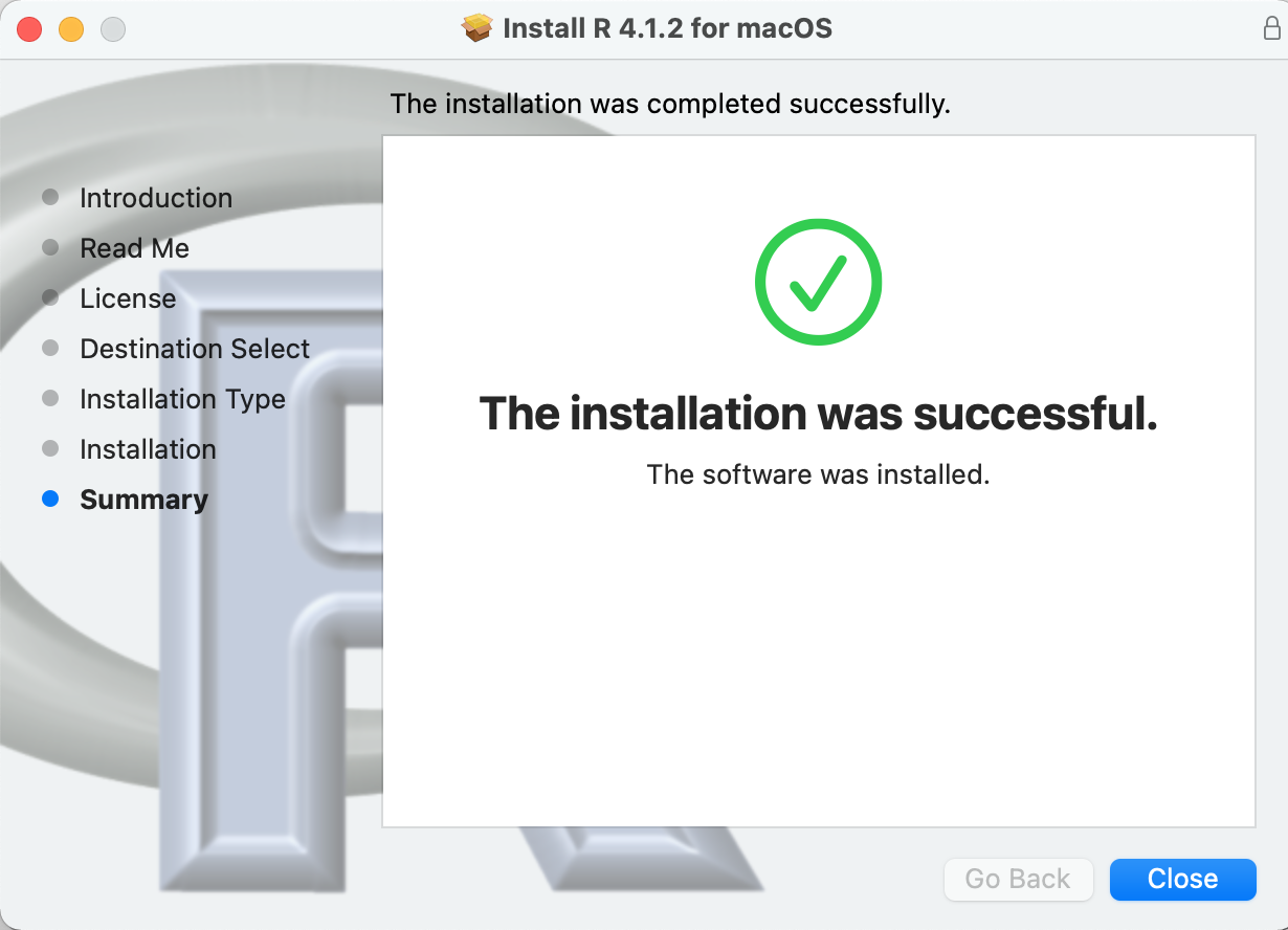
Figure 1.1: You should download the R distribution that is appropriate for you machine. It is a very quick install.
Download the version of R that’s right for you. I’m guessing either MacOS or WindowsOS. The disk image will go to your Downloads folder. If you are downloading the Linux version, you get to teach this class.
Follow the onscreen instructions. It’s a quick download.
1.2 Downloading RStudio
Go back to the RStudio download page and now click the big, blue button to get RStudio. Again, follow the onscreen instructions.
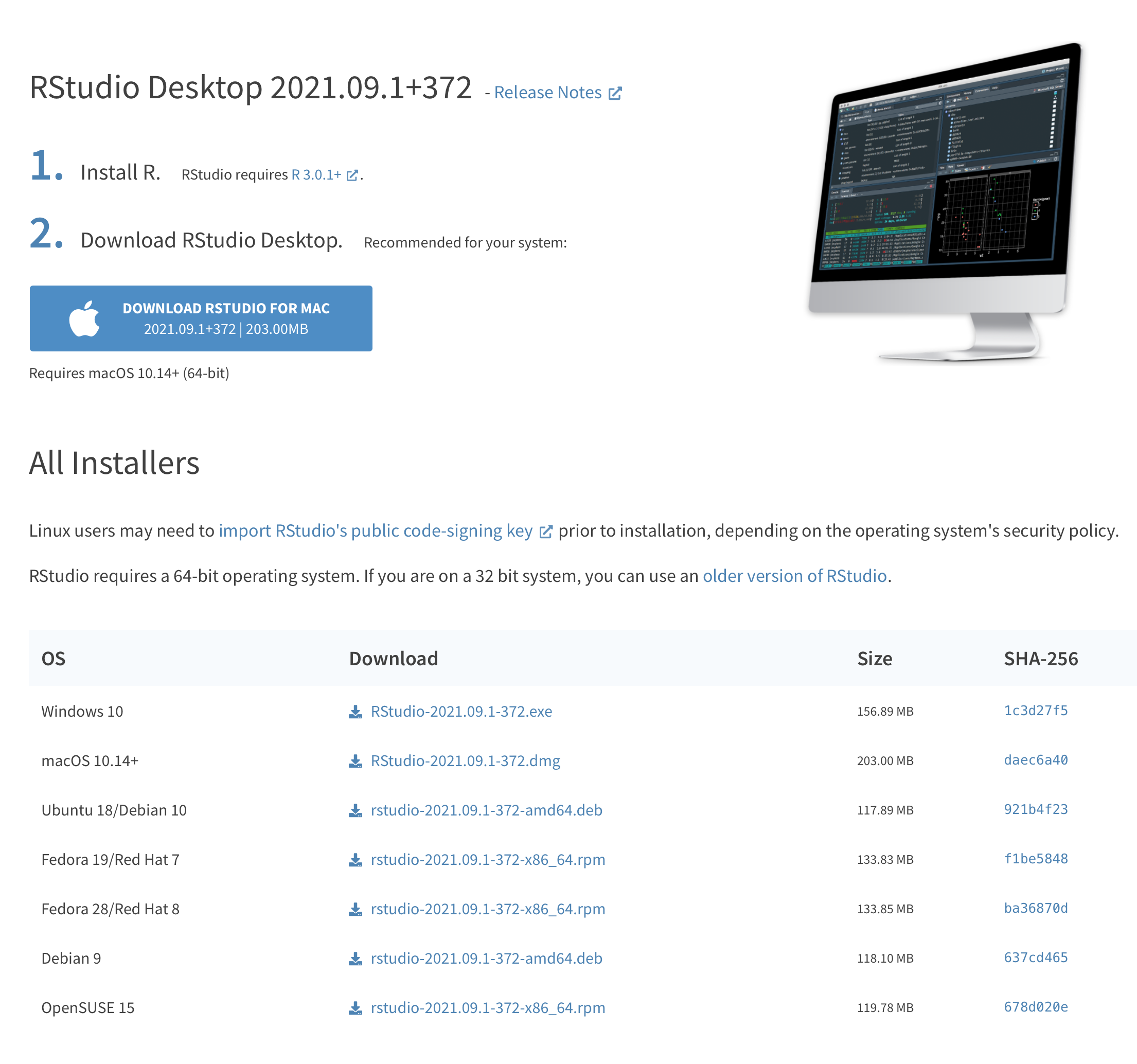
Figure 1.2: Also download the version of RStudio that works with your laptop. This is also a quick install.
1.3 A Tour of RStudio
We’ll spend time in class going over RStudio and where to find what you need. The folks at Software Carpentry have put together a good introduction to R and RStudio.
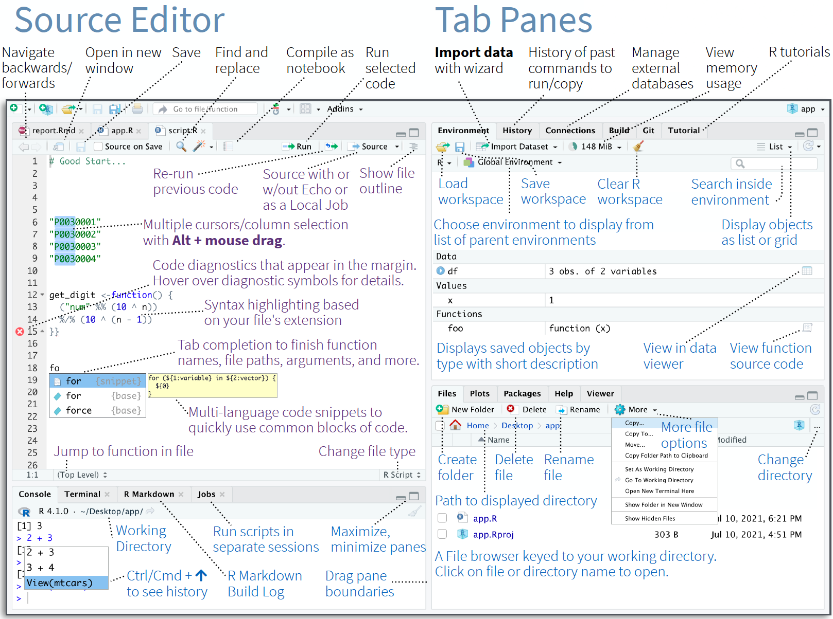
Figure 1.3: RStudio lets you write your code, view your data, see your output, manage your R packages, and many other things. We are only going to see the very basics. Source: RStudio IDE Cheatsheet
RStudio gives us space to write out code, whether that is a script or a notebook, manage our packages, see our output, access the R command line, and even access our computer’s own command line, among many other features. We won’t need to worry about a lot of the details this evening.
When you first open RStudio, you will see three panels:
- The interactive R console/Terminal (entire left)
- Environment/History/Connections (tabbed in upper right)
- Files/Plots/Packages/Help/Viewer (tabbed in lower right)
Let’s take a tour around some of the important features of RStudio.
1.3.1 R as a Calculator
The R Console is accessible in the bottom left window of RStudio. This is where you can interact with R from the command line. You can also see the messages and warnings that R will give to you when you run your code. On a Mac, you can access Terminal from here.
Go ahead and use R as a calculator. The <- assigns 2 to X. You could use an =, but that is not very R-like.
x <- 2
x * 2
#> [1] 4
1.3.2 Installing Packages
Packages let us add extra functionality to R. They are installed with the install.packages function and loaded with the library function, once per session. The code for this is:
install.packages("package_name")
library(package_name)
For example, you could type the following into the R Console:
install.packages("tidyverse")
library(tidyverse)
You will have now installed the tidyverse on your computer and allowed you to access everything in it with the library function. Why do we want the tidyverse package? This has the good stuff.
Packages are free, open-source software that are maintained by the R community and then posted to a special server called CRAN. You can also type out these commands in code. For example,
installed.packages() #What packages are installed?
update.packages() #Update my packages!
remove.packages("packagename") #Remove a package
You don’t have to do this from the Console. In the bottom right of RStudio, you’ll see the Files/Plots/Packages/Help/Viewer windows. Click on Packages. You can click on Install and search for the package that you want. Again, you only need to do this once. Once the package is on your computer, it lives there. You can also click Update to update your packages. Finally, you can scroll and see what you have installed.
1.3.3 The Global Environment
There is an important panel in the upper right of RStudio called Environment. In particular, we can see the Global Environment. This panel shows you all of the data sets that you have in memory, variables that you have created, etc. Let’s add something to it. Type this line into your script
c <- carsI have now assigned a data set that comes pre-installed with R, called cars, to a data frame in memory that I’ve called c. I did this using <-, which is the R assignment operator that I used above in the calculator example. I can check and see exactly what I’ve created using the class function
class(c)
#> [1] "data.frame"
Turns out, I’ve put this data into something called a data.frame. More on that in Section 2 of our notes.
1.3.4 Searching for Help
You can also get help directly in RStudio. Let’s go back to the bottom right of RStudio and click on Help. The bar with the arrows has a search bar. You can type in a package that you’ve installed, or a function that you want to know more about, and get the standard R help window.
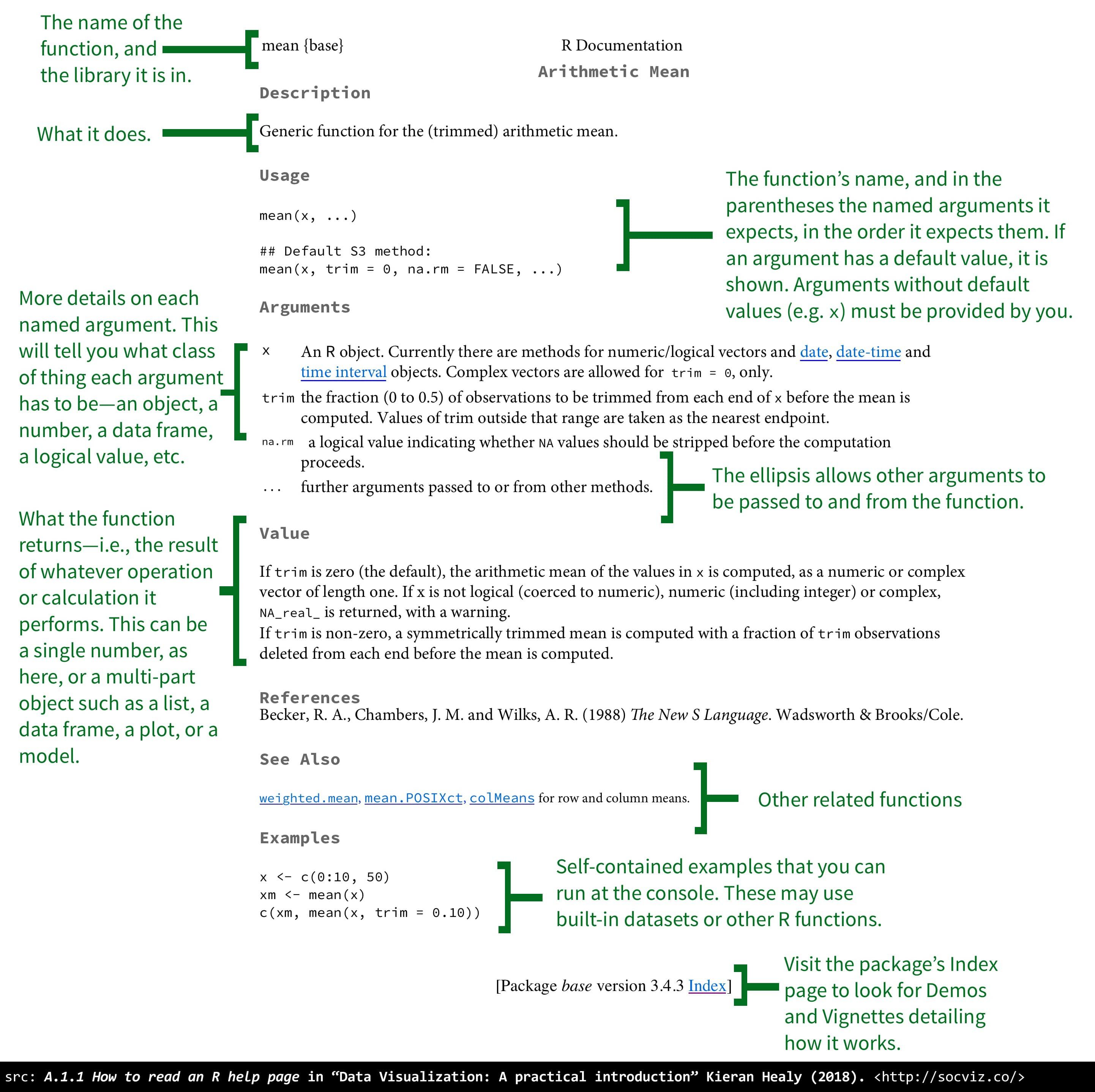
Figure 1.4: Good to know how to actually read these help files!
1.4 Organize Yourself
OK, before we do anything else, we need to get organized. When writing code, doing data work, anything on a computer, it is very important to know where your stuff lives. Let’s start by setting up your folders for this class. We’ll then create an R Project.
- Create a folder called elon-r-datacamp. This folder could live in your Documents folder on your computer.
- Inside this folder, create an RStudio project. What are projects? This is the file that you will open every time you work on something for that project and gives you a home base. You can create a new project in the upper right of RStudio. Check out Chapter 8 of R For Data Science for the details. Name the project elon-r-datacamp
- Inside this folder, create additional folders, such as data and output. Avoid spaces, capital letters, and special characters in your names.
Go to the bottom right of RStudio and click on Files. You should see the folder that your project file is in.
We are now going to start creating files and loading in data to see what R can do. We’ll talk about relative vs. absolute file paths. The R Notebook example for this course also goes over this material.
1.5 R Scripts
Any commands that you write in the R console can be saved to a file to be run again. Files that contain R code like this are called R scripts. R scripts have .R at the end of their names to let you know what they are. You can run it line-by-line, or all at once. Once you open files, such as R scripts, an editor panel will also open in the top left of RStudio.
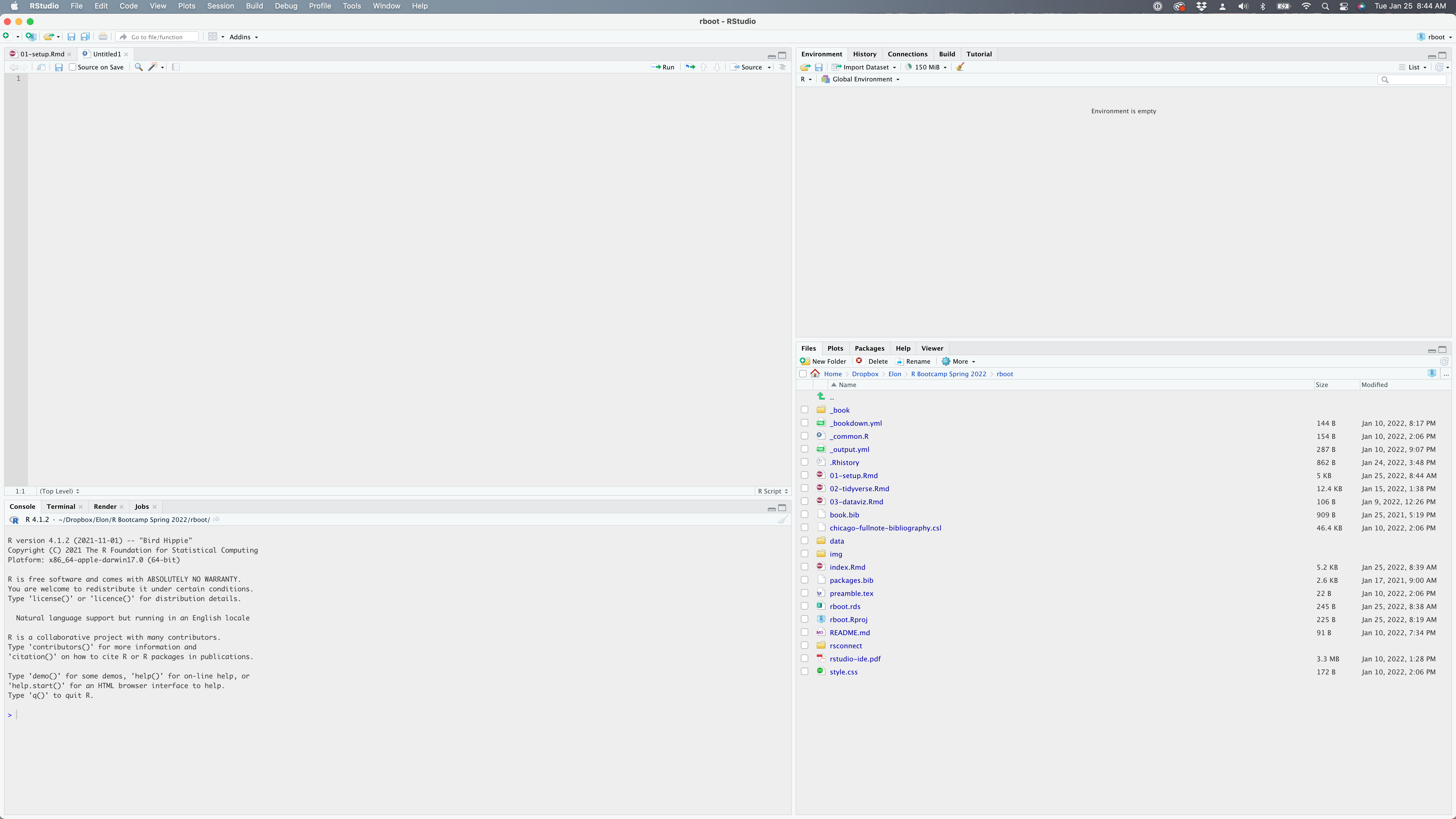
Figure 1.5: I have opened up a new R Script from the File menu. You can see my my current working folder on the bottom right. My global environment is currently empty.
Go under File -> New File at the top of R Studio and create a new script. Note the keyboard shortcut. You can find more keyboard shortcuts here.
Let’s look at the example R script from our course Github page and work together to add some code to your script. You’ll use R scripts a lot. They are the main way to organize your code and create a step-by-step process for importing, cleaning, and analyzing data. In fact, each step of your workflow will likely get its own script.
When we’re done, save your r script in elon-r-datacamp as r-script-example.r
1.6 R Notebooks
R scripts let us write and comment our code. But, what if we want to create a report to show someone? We can send people our R script, but there might be a better way. R Notebooks mix R code and Markdown formatting syntax to create HTML, PDF, and MS Word documents.
For more details on using R Markdown, see http://rmarkdown.rstudio.com or Chapter 27 of R for Data Science for the basics. For much more, here’s a complete book on Markdown and R.
In short, R Markdown lets us combine our code with a document that displays the code’s output, such as tables and graphs. There’s no need to do your code one place and then put things into a Word or Google Doc. But, RStudio allows us to mix Markdown, which creates the formatted text in our document, with R, which does the statistical analysis.
Markdown itself has nothing to do with R - it is a way to format a document using plain text.
There’s an example of an R Notebook on our Github page. We can open up a new R Notebook under File -> New File. Let’s do that and work through an example together.
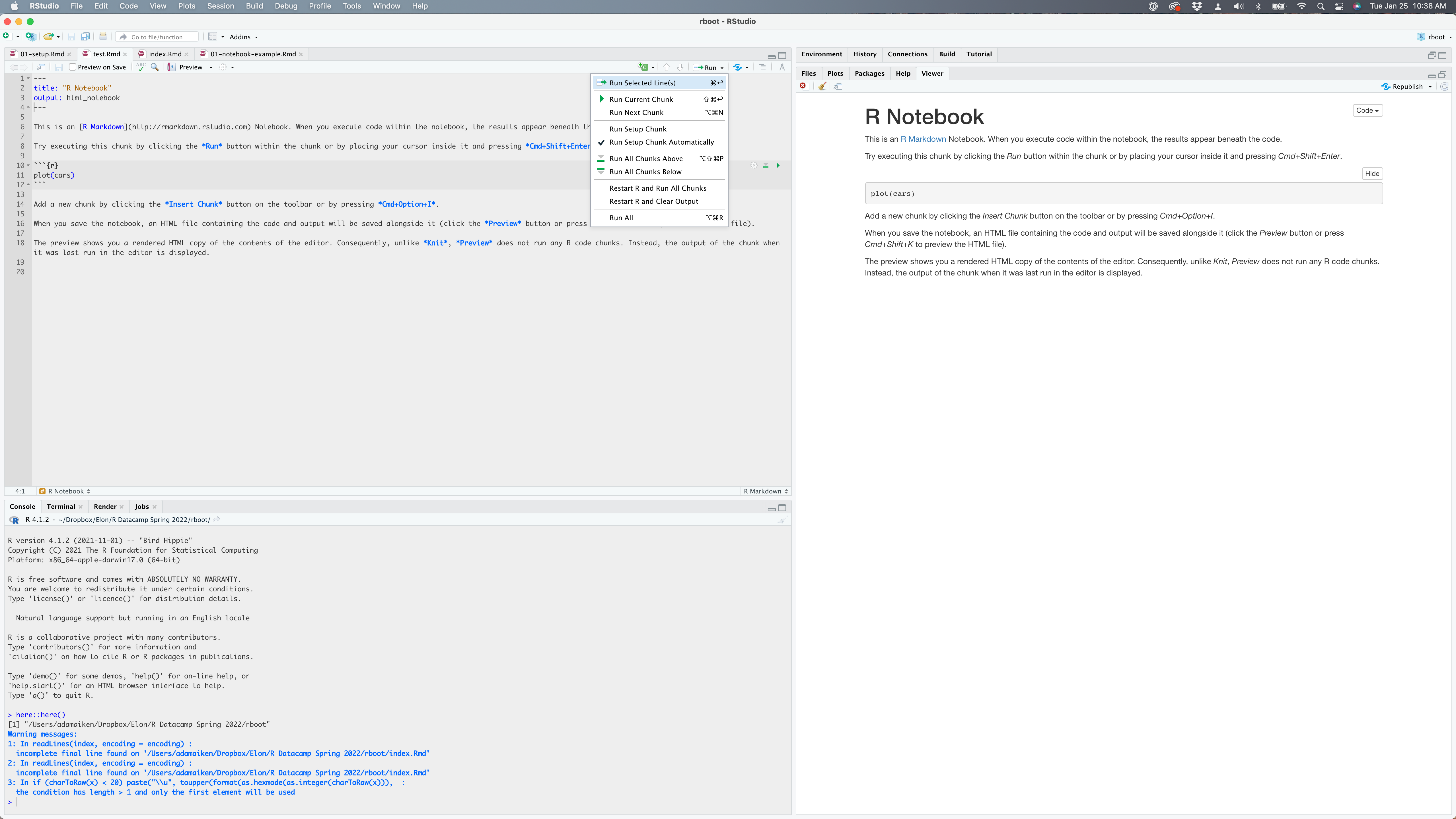
Figure 1.6: An R Notebook when you first open it. My cursor is over all of the run options. Note the keyboard shortcuts.
When you create an R Notebook for the first time, you’ll see a button at the top of the code window called Preview. Click that. RStudio is now going to ask you to save your .Rmd file. Save this R Notebook in your elon-r-datacamp folder as my-class-notebook.Rmd.
The Viewer panel on the right should now have a preview of this notebook. How does it know what to show you? There was already some markdown code in the new file!
Click the down arrow next to Preview. You’ll see an option Knit to HTML. We can also knit, or render, the document in the output of our choosing. For now, we will create an HTML file from this document. You can also create a PDF or a Word file. You can also find these options under the Preview menu.
Once you Knit to HTML, the Preview button will turn into Knit. There will also be an HTML file in your folder that contains your output. This is the file that you can share with someone.
While R Notebooks use Markdown, they are not the same as R Markdown documents. Go under the File menu. See how you can create an R Notebook and an R Markdown document? You want an R Notebook for what we’re doing.
Finally, there is a new method for doing all of this called Quarto. It also uses Markdown and is a powerful way to create documents. You’ll notice that Quarto Document is actually the second option under File::New File.
1.6.1 Chunks
When you execute code within the notebook, the results appear beneath the code. Try executing this chunk by clicking the Run button within the chunk or by placing your cursor inside it and pressing Cmd+Shift+Enter on a Mac or Ctrl+Shift+Enter on a PC.
summary(cars)
#>      speed           dist
#>  Min.   : 4.0   Min.   :  2.00
#>  1st Qu.:12.0   1st Qu.: 26.00
#>  Median :15.0   Median : 36.00
#>  Mean   :15.4   Mean   : 42.98
#>  3rd Qu.:19.0   3rd Qu.: 56.00
#>  Max.   :25.0   Max.   :120.00
Here’s another chunk of code you can try.
plot(cars)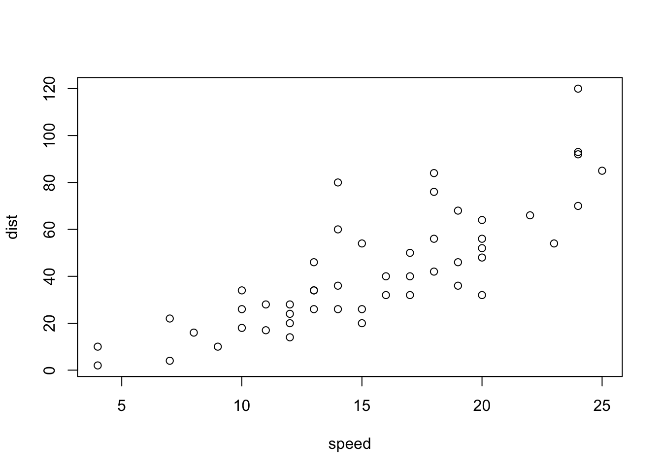
Add a new chunk by clicking the Insert New Code Chunk button on the toolbar or by pressing Cmd+Option+I on a Mac or Ctrl+Option+I on a PC. You will then type your R code inside.
When you save the notebook, an HTML file containing the code and output will be saved alongside it. You can click the Preview button, or press Cmd+Shift+K on a Mac or Ctrl+Shift+K on a PC, to preview the HTML file.
In R Notebooks, you need to first run the code chunks in order to have them show up in the Preview and final, knitted documents. The preview shows you a rendered HTML copy of the contents of the editor. Consequently, unlike Knit, Preview does not run any R code chunks. Instead, the output of the chunk when it was last run in the editor is displayed.
1.6.2 YAML Header
The options at the very top are called a YAML header. It contains options for the entire document. We are keeping things simple for now, but there’s a lot you can include up there. When you open up a blank Notebook, you get this YAML:
---
title: "R Notebook"
output: html_notebook
---
After you Knit to HTML, the YAML header changes to:
---
title: "R Notebook"
output:
  html_document:
    df_print: paged
---
Changing the title option changes the title of the HTML file that R Studio generates. We can add other options to, like author: and date:. Try this and then Preview your notebook.
There are all kinds of things you can add to the YAML header to customize and format your output. If you know HTML and CSS, then you can really get creative.
1.6.3 More On Chunks
If you’re looking at my code, you’ll notice that I have some text in between the curly brackets in my chunks. These are chunk options. They let me tell R specific instructions to follow when running the code inside that chunk. First, r just means that I have R code inside the chunk. RStudio can actually run other languages, such as SQL and Python. Then, the text that follows is the name of the chunk. Keep you names short, but informative, with no spaces or special characters. Here’s an example without the curly brackets:
r setup, include=FALSENote that there is no comma between r and setup, the name that I gave this chunk. I like to have a setup chunk at the top of my code that contains commands that are relevant to the entire document. I’ll usually load the libraries (packages) that I want there. All code chunks must have different names, so if you copy and paste chunks, but forget to change the names, you’ll get an duplicate label error at the top of your notebook.
Options go after the comma. The first, include=FALSE, means to not include this code in the R Notebook output, but to still run the code. If you set this to FALSE, then the code will not show up in the final document. This might be what you want in your final report.
You can also turn off warning, error, and message. Set warning=FALSE to keep the warning messages out of your final document. Some code generates messages, such as read_csv. You can remove these from the document output by setting message=FALSE.
Other important options include things that affect figure output, such as size or alignment.
You can read more about all of the options here.
1.7 Folders, Paths, and Data
Let’s finally get some external data in R. In Section 2 of our notes, we’ll talk about how to clean, alter, and summarize our data. In Section 3, we’ll discuss making graphs.
Inside of the data folder, save the ncbreweries.csv file from our course Github page. We are going to use this data in our examples. But, before we load in our data, we need to talk about file paths.
Let’s install and load another package, here. The package here will help us keep things organized and lets us avoid typing out a bunch of file paths. You can add this code to a new chunk in your R Notebook:
install.packages("here")
library(here)
here::here()
When I used the here::here() command above, R looked through my folders until it found my RStudio project file, which lives in my elon-r-datacamp folder. My relative path is .../elon-r-datacamp/data if I want to load in a data file.
Why do this? All of your computers have different user names, so you can’t just copy and paste the full path names! My files actually live in the /Users/adamaiken/elon-r-datacamp folder. Your folder obviously won’t have this name. But, if we all have the same folder names below our main folder, then we can all use the same relative file paths. This will mean that you can share code, without changing path names to load in data.
I know this is all kind of confusing, but it will get easier with examples and practice. Let’s load in some actual data to see how this works with the here package. Again, add this code to a new chunk in your Notebook.
Remember, here says that it will start looking in the elon-r-datacamp folder. I then use the here::here() function to navigate down folders, into data, until I find my .csv file with breweries data.
here is making it easy for us to write read_csv("/Users/adamaiken/elon-r-datacamp/data/ncbreweries.csv"). In fact, I’ll try that now on my machine, just to show you that it works.
nc_brew2 <- read_csv("/Users/adamaiken/elon-r-datacamp/data/ncbreweries.csv")There’s another way to do this, without using here::here. This file lives in /Users/adamaiken/elon-r-datacamp/. By default, R Notebook files start their relative path in the same folder that they live in. So, if my .csv file lives in the data folder in the directory that my .Rmd file lives in, I can access it like this.
nc_brew3 <- read_csv("data/ncbreweries.csv")When I don’t use here::here, path names are relative to where a particular .Rmd file lives, rather than where my project file lives. I like using here::here, since it starts where my project file lives.
By the way, we’ve now loaded in the same data set three times to our global environment! Take a look on the right.
Knowing how to set up your data to be machine readable is critical. How should you set up an Excel file to get it into software like R or Python?
Finally, let’s load the data in a fourth time. Instead of worrying about where it is stored locally, you can also just go and grab data that stored on the web, like in my Github page.
nc_brew4 <- read_csv("https://raw.githubusercontent.com/aaiken1/elon-r-datacamp/main/data/ncbreweries.csv")1.8 Markdown Formatting
Markdown uses plain text to format our documents. So, no buttons or GUI to select bold or italics. We’re using Markdown in our R Notebooks, as we’ve seen above.
Lots of other programs use Markdown, so learning it is useful. If you are an Apple fan and read Daring Fireball, John Gruber and Aaron Swartz created the Markdown language.
See Chapter 27.3 of R For Data Science for more on how to create headers, lists, and tables in Markdown.
Here are some common formats for bold, italics, headers, lists, etc. Markdown is actually translating your “code” to HTML in the background.
Text formatting
------------------------------------------------------------
*italic* or _italic_
**bold** __bold__
`code`
superscript^2^ and subscript~2~
Headings
------------------------------------------------------------
# 1st Level Header
## 2nd Level Header
### 3rd Level Header
Lists
------------------------------------------------------------
* Bulleted list item 1
* Item 2
* Item 2a
* Item 2b
1. Numbered list item 1
1. Item 2. The numbers are incremented automatically in the output.
Links and images
------------------------------------------------------------
<http://aaiken1.github.io>
[linked phrase](http://aaiken1.github.io)

Tables
------------------------------------------------------------
First Header | Second Header
------------- | -------------
Content Cell | Content Cell
Content Cell | Content Cell