Chapter 3 Aseet Price Modelling and Stochastic Calculus

Now that we are armed with a solid background in Probability theory we can start to think about how to model the evolution of an asset. To kick things off we will consider two time points \(t \to t+\delta t,\) where, as is customary, we think of \(\delta t\) as being a small time interval. Recall that time is measure in years and so to \(3\) significant figures we have

\[ \begin{aligned} \delta t &= 1 \, {\rm{day}}\,\,= \frac{1}{365}\approx 0.00274\, \, & \\ \delta t &= 1 \, {\rm{hour}}\,\,= \frac{1}{24 \times 365}\approx 0.000114\, \, & \\ \delta t &= 1\, {\rm{minute}}\,\,= \frac{1}{60 \times 24 \times 365}\approx 0.00000190. \end{aligned} \]

Thus anything \(\le\) 1 day can be view as small here. If our investment was cash in a risk free back (offering the risk free rate \(r\)) then, if we let \(D(t)\) denote the amount of cash in the bank at time \(t\) then we can be absolutely certain that at time \(t+\delta t\) this will have grown in the following manner

\[ D(t)\to D(t+\delta t)=D(t)+r\delta t D(t), \]

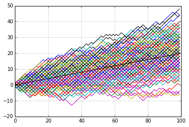
i.e., the investment earns an additional \(r\delta t D(t)\) in interest. Obviously, things are entirely different if our investment is in some risky asset; a stock, commodity, currency etc… But let us use the deterministic model above as a guide for what we can say about the future outcome. We are all familiar with the jagged plots of stock market behaviour from the financial pages; typical examples are given in the picture below.

We notice that even though the risky asset path evolves randomly over this the time period, it is possible to detect a general trend as illustrated by the green trend line. At a glance the trend lines for the two assets have have the same slope; stated in financial language we say that the two assets both have the same expected growth rate. However, the fluctuations around these trend lines are much wilder in the example on the right; the example on the left sticks shows variability but does not stray too far away from the trend line; in financial language we say that the asset depicted on the right is more volatile than the one on the left. Thus, from an investors point of view the asset on the left hand side would be the preferred choice. Given that we see such patterns in the short term behaviour of our assets we certainly need to incorporate these feature into our model. That said, we propose the following approach:

\(\diamond\) We’ll chop \([0,T]\) into subintervals and model the change over this short time interval as a trend together with a random fluctuation.

\(\diamond\) We choose \(n\) to be a large positive integer and let \(\delta t = \frac{T}{n},\) then scan across the interval like:

\[ 0=t_{0}<\delta t = t_{1}<2\delta t = t_{2}<\cdots <i\delta t = t_{i}<(i+1)\delta t=t_{i+1}<\cdots n\delta t=T. \]

\(\diamond\) Across each sub interval we propose:

\[ S_{i+1}=S_{i}+\mu\delta t S_{i}+\sigma\sqrt{\delta t} S_{i}Z_{i},\quad {\rm{where}}\,\,\, Z_{i}\sim N(0,1), \quad i=0,1,\ldots, n-1. \]

The picture below illustrates the idea.

We note that the opening two terms simply emulate the deterministic model (with the risk free rate replaced with the drift rate of the asset) but the final component is there to capture the random nature of the asset. In keeping with the well known principle (past performance is no indicator of the future) we will assume that as time evolves the standard normal random variable \(Z_{1},Z_{2},\ldots\) are independent. The parameter \(\sigma\ge 0\) is the volatility and its size determines the strength of the fluctuations around the drift rate.

There are a couple of natural questions that I thin k spring to mind when we review this model

1. Why is there a \(\sqrt{\delta t}\) factor in the random contribution?

ANS: This is to do with something that will come later and that is the generalization of this model from discrete time points to the continuous setting. In order to do this we will be examining the limit \(\delta t \to 0\) and the \(\sqrt{\delta t}\) is there so we can do this sensibly. For a bit more detail you may recall that if \(X\) is a random variable with variance \(\sigma^{2}\) then if we scale \(X\) by a positive quantity \(a\) then the variance of \(aX\) is \(a^{2}\sigma^{2}.\) With this fact in mind you can see that, under our model - given the \(\sqrt{\delta t}\) factor - the variance of the asset will scale linearly with time; this, in turns out, is a desirable feature of the model.

2. Why use standard normal random variables?

ANS: To understand the reason for this you need to consider how we will be using the model (this will come apparent when we explore it in some detail). In getting to the point where we have an expression for the asset price at a particular time \(t\) we will reach a point where we consider a large sum of i.i.d normally distributed random variables for which is itself normally distributed. Well, if we took another sequence of i.i.d random variables (with zero mean and unit variance) then due to the central limit theorem we would still arrive at the same result. Once you understand the passage from the discrete model to the continuous model you can verify this for yourself.

3.1 Derivation of the Continuous Time Model

We will now use the discrete model to find a continuous time expression for the value of the asset at time \(t \in [0,T].\) One way to do this is to consider the interval \([0,t]\) and partition it by choosing a natural number \(L,\) which we use to define the small time increment \(\delta t = t/L\) and use our proposed model to get a price for \(S_{L}=S(t).\) The picture below illustrates the situation.

Of course, by doing it like this we only arrive at that price from a sample of \(L\) previous values. To make this continuous, so that the whole path of values up to time \(t\) is captured we have make sure that

\(\diamond\) \(\delta t \to 0\) and \(L \to \infty\) in such a way that we always keep \(L\delta t =t.\)

\(\,\)

Let us start by getting the expression for \(S(t)\) from the fixed \(L\) samples. We recall that our model states that

\[ S_{i+1}=S_{i}(1+\mu \delta t +\sigma \sqrt{\delta t}Z_{i}),\quad Z_{i}\sim N(0,1). <center>\]

We make the obvious observation that, over each time increment \(\delta t,\) the previous asset price gets multiplied by \((1+\mu \delta t +\sigma \sqrt{\delta t}Z_{i})\) to get the new price. So it all rolls out as follows

\[ S_{1}=S_{0}(1+\mu \delta t +\sigma \sqrt{\delta t}Z_{0}) \]

then

\[ S_{2}=S_{1}(1+\mu \delta t +\sigma \sqrt{\delta t}Z_{1})=S_{0}(1+\mu \delta t +\sigma \sqrt{\delta t}Z_{0})(1+\mu \delta t +\sigma \sqrt{\delta t}Z_{1}) \]

and then

\[ S_{3}=S_{0}(1+\mu \delta t +\sigma \sqrt{\delta t}Z_{0})(1+\mu \delta t +\sigma \sqrt{\delta t}Z_{1})(1+\mu \delta t +\sigma \sqrt{\delta t}Z_{2}) \]

and so on, you get the picture, until we reach time step \(L\) (coinciding with time \(t\)) and we end up with

\[ S(t)=S_{L}=S_{0}\prod_{i=0}^{L-1}(1+\mu \delta t +\sigma \sqrt{\delta t}Z_{i}). \]

The product term is not the easiest to deal with so, a nice trick is to take logs to turn it into a sum that we can examine; before we do so we first divide through by \(S_{0}\) and consider instead:

\[ \ln\left(\frac{S(t)}{S_{0}}\right)=\sum_{i=0}^{L-1}\ln(1+\mu \delta t +\sigma \sqrt{\delta t}Z_{i}). \tag{3.1} \]

As we’ve made clear, we are interested in what happens when \(\delta t \to 0\) in such a way that \(L\to \infty\) to ensure \(L \delta t =t.\) We keep in mind that \(L\) will get large but mainly focus on the fact that \(\delta t\) is approaching zero. Specifically, we can take advantage of the following approximation of the logarithm function

\[ \ln(1+\epsilon)\approx \epsilon -\frac{\epsilon^{2}}{2},\quad {\rm{for}}\,\,{\rm{small}}\,\,\epsilon. \]

At this point I should mention that the approximation above is naturally quoted in the deterministic case, it is not immediately obvious if it holds with the same strength when random variables are involved- note in our case the \(\epsilon\) would be \(\mu \delta t +\sigma \sqrt{\delta t}Z_{i}\). It turns our that we can, in this case, but I will not go into the technical details (you are left to ponder this for yourself in a quiet moment). Accepting that the approximation can be employed we have

\[ \ln(1+\mu \delta t +\sigma \sqrt{\delta t}Z_{i})\approx \mu \delta t +\sigma \sqrt{\delta t}Z_{i}-\frac{(\mu \delta t +\sigma \sqrt{\delta t}Z_{i})^{2}}{2}. \]

Now the next assumption/simplification that we are going to make rest on the fact that we are allowing $t $ to approach zero, and as such we make the decision to ignore any powers of \(\delta t\) that are higher than \(1\) (the linear term). Thus, upon expanding the square term in the denominator we ignore the \(\mu^{2}(\delta t)^{2}\) term AND the \(2\mu\sigma Z_{i}(\delta t)^{\frac{3}{2}}\) term and KEEP ONLY the \(\sigma^{2}Z_{i}^{2} \delta t\) term. This will always be our rule, throughout this course, when dealing with small increments of time. Thus, implementing it here gives:

\[ \ln(1+\mu \delta t +\sigma \sqrt{\delta t}Z_{i})\approx \mu \delta t +\sigma \sqrt{\delta t}Z_{i}-\frac{\sigma^{2}\delta t Z_{i}^{2}}{2}. \]

In particular, going back to @(eq:one), we have

\[ \begin{aligned} \ln\left(\frac{S(t)}{S_{0}}\right)\approx \sum_{i=0}^{L-1}\left(\mu \delta t +\sigma \sqrt{\delta t}Z_{i}-\frac{\sigma^{2}\delta t Z_{i}^{2}}{2}\right)&=\sum_{i=0}^{L-1}\mu \delta t+ \sum_{i=0}^{L-1}\left(\sigma \sqrt{\delta t}Z_{i}-\frac{\sigma^{2}\delta t Z_{i}^{2}}{2}\right) \end{aligned} \]

Observe the first term can be simplified

\[ \sum_{i=0}^{L-1}\mu \delta t = \mu L\delta t =\mu t \]

and so we have

\[ \begin{aligned} &\quad\quad \quad\quad \quad\quad \quad \ln\left(\frac{S(t)}{S_{0}}\right)\approx \mu t+ \sum_{i=0}^{L-1}Y_{i},\\ &{\rm{where}}\,\,\, Y_{i}:= \sigma \sqrt{\delta t}Z_{i}-\frac{\sigma^{2}\delta t Z_{i}^{2}}{2}, \,\,\,{\rm{are}}\,\,\, i.i.d \,\,\, {\rm{random}}\,\, {\rm{variables}}\,\,\, (Z_{i}\sim N(0,1))\end{aligned} \tag{3.2} \]

So we now have on our hands a large sum of \(i.i.d\) random variables each sharing the same mean and same variance. Since \(Z_{i}\sim N(0,1),\) we have \(\mathbb{E}[Z_{i}]=0\) and \(\mathbb{E}[Z_{i}^{2}]=1\) this allows us to conclude that the shared mean of the \(Y_{i}\) random variable is

\[ \mathbb{E}[Y_{i}]=\mathbb{E}\Bigl[\sigma \sqrt{\delta t}Z_{i}-\frac{\sigma^{2}\delta t Z_{i}^{2}}{2}\Bigr]=\sigma \sqrt{\delta t}\mathbb{E}[Z_{i}]-\frac{\sigma^{2}\delta t}{2}\mathbb{E}[Z_{i}^{2}]=-\frac{\sigma^{2}\delta t}{2}. \]

We can compute the shared variance of the \(Y_{i}\) can be computed using the formula

\[ \begin{aligned} {\rm{var}}(Y_{i})=\mathbb{E}[Y_{i}^{2}]-\mathbb{E}[Y_{i}]^{2}& = \mathbb{E}\Biggl[\left(\sigma \sqrt{\delta t}Z_{i}-\frac{\sigma^{2}\delta t Z_{i}^{2}}{2}\right)^{2}\Biggr]-\frac{\sigma^{4}}{4}(\delta t)^{2}\\ &=\mathbb{E}\Bigl[\sigma^{2} Z_{i}^{2}\delta t - \sigma^{3}Z_{i}^{3}(\delta t)^{\frac{3}{2}}+\frac{\sigma^{4}Z_{i}^{4}}{4}(\delta t)^{2}\Bigr]-\frac{\sigma^{4}}{4}(\delta t)^{2}. \end{aligned} \]

Now recall our decision that we ignore all powers of \(\delta t\) that are greater than one. This means that, for our purposes, the shared variance is given by

\[ {\rm{var}}(Y_{i})=\mathbb{E}[\sigma^{2} Z_{i}^{2}\delta t]=\sigma^{2}\delta t. \]

We can now bring in the famous central limit theorem to conclude that the large sum of the \(Y_{i}\) random variables (each with mean -) and variance ^{2}t) is approximately a normal variable, specifically

\[ \sum_{i=0}^{L-1}Y \approx \sim N\left(-L\frac{\sigma^{2}\delta t}{2},L\sigma^{2}\delta t\right)= N\left(-\frac{\sigma^{2}t}{2},\sigma^{2}t\right) \]

where we have used the fact that \(L\delta t=t.\) In the limit as \(L\to \infty\) and \(\delta t \to 0\) (such that $Lt=t) the above become an exact statement (using the central limit precisely) and thus, in view of @(eq:two), we can conclude that

\[ \ln\left(\frac{S(t)}{S_{0}}\right)\sim N\left(\left(\mu-\frac{\sigma^{2}}{2}\right)t,\sigma^{2}t\right). \tag{3.3} \]

Based on the above arguments we can propose the following continuous time model for the evolution of our asset

\[ \ln\left(\frac{S(t)}{S_{0}}\right)=\left(\mu-\frac{\sigma^{2}}{2}\right)t+\sigma\sqrt{t}Z,\quad Z\sim N(0,1). \]

Exponentiating, we have

\[ S_{t}=S_{0}\exp\left(\left(\mu-\frac{\sigma^{2}}{2}\right)t+\sigma\sqrt{t}Z\right),\quad Z\sim N(0,1). \tag{3.4} \]

We remark that we kicked off this development with the aim of targeting the time \(t\) by considering the fine partition of the interval \([0,t]\). Of course there the time \(t\) is arbitrary but also there is nothing special about choosing the interval \([0,t].\) For instance, if we choose \(0<t_{1}<t_{2}<T\) and repeat the above analysis with the interval \([t_{1},t_{2}]\) in place of \([0,t]\) then we will discover the analogous formula to (3.3), i.e,

\[ \begin{aligned} \ln\left(\frac{S(t_{2})}{S(t_{1})}\right)&\sim N\left(\left(\mu-\frac{\sigma^{2}}{2}\right)(t_{2}-t_{1}),\sigma^{2}(t_{2}-t_{1})\right)\\ &\implies S(t_{2})=S(t_{1})\exp\left(\left(\mu-\frac{\sigma^{2}}{2}\right)(t_{2}-t_{1})+\sigma\sqrt{t_{2}-t_{1}}Z_{1}\right),\quad Z_{1}\sim N(0,1). \end{aligned} \]

Of course, if we add another point \(t_{3}\) so that \(0<t_{1}<t_{2}<t_{3}<T\) then we can move onto the next subinterval \([t_{2},t_{3}]\) to yield:

\[ \begin{aligned} \ln\left(\frac{S(t_{3})}{S(t_{2})}\right)&\sim N\left(\left(\mu-\frac{\sigma^{2}}{2}\right)(t_{3}-t_{2}),\sigma^{2}(t_{3}-t_{2})\right)\\ &\implies S(t_{3})=S(t_{2})\exp\left(\left(\mu-\frac{\sigma^{2}}{2}\right)(t_{3}-t_{2})+\sigma\sqrt{t_{3}-t_{2}}Z_{2}\right),\quad Z_{2}\sim N(0,1). \end{aligned} \]

For these two non-overlapping intervals \((t_{1},t_{2}),\) \((t_{2},t_{3})\) the standard normal random variables \(Z_{1},Z_{2}\) are independent and this gives us a means of describing the path of the asset across an increasing sequence of time points. The picture below illustrates the first two steps as described above.

Generalizing this we can describe we can describe the path of the asset price over a sequence of increasing time points

\[ 0=t_{0}<t_{1}< t_{2}<\cdots <t_{M}=T \]

in a recursive manner using the formula

\[ S(t_{i+1})=S(t_{i})\exp\left(\left(\mu-\frac{\sigma^{2}}{2}\right)(t_{i+1}-t_{i})+\sigma\sqrt{t_{i+1}-t_{i}}Z_{i}\right),\quad {\rm{for}}\,\, i=0,1,\ldots, M-1 \]

where the sequence \(Z_{i}\sim N(0,1)\) are independent. This feature is potentially very valuable if we need to simulate potential paths of our asset price.

3.2 Stochastic Processes, Random Walks and Brownian Motion

Now is the right time to introduce the notion of a stochastic process. This is not as daunting as the notation suggests, put simply it is just a random variable that depends upon time. There are two things to consider

\(\bullet\) If we are considering time in discrete ‘ticks’ say \(0=t_{0}<t_{1}<\cdots,\) then we are investigating a so-called discrete stochastic process \(X_{0},X_{1},\ldots\) basically a sequence of random variables indexed to ticks of time.

\(\bullet\) If we are considering a process that evolves continuously, typically \(t \in [0,\infty)\) then we are investigating a so-called continuous stochastic process \(\{X_{t}:t \in [0,\infty)\}.\)

When studying stochastic processes it is natural to investigate the behaviour over a given time interval e.g. between \(t_{k}\) and \(t_{k+n}\) for a discrete process or between times \(s\) and \(t\) \((s<t)\) for a continuous process. When we do this we talk of the increment of the stochastic process

\[ X_{k+n}-X_{k} \,\,\, {\rm{(discrete}}\,\,{\rm{increment)}}\quad {\rm{and}}\,\,\, X_{t}-X_{s}\,\,\, {\rm{(continuous}}\,\,{\rm{increment),}} \]

the increments are of course random variables in their own right.

We are going to focus particularly on one of the most famous stochastic processes, the so-called Brownian motion. You will probably have encountered Brownian motion is science from high-school, it is named in honour of the Scottish botanist Robert Brown who, in 1826, observed the irregular motion of pollen particles suspended in water. He noted two observations

1. the path of a given particle is very irregular with no tangent.

2. the motion from one point to the next appears to be independent all previous movements.

In 1900 Louis Bachellier, emulating Brown somewhat, attempted to mathematically describe the stock market in terms of random fluctuations. From the 1920s onwards Norbert Weiner’s work really established the mathematical theory behind these observations. The formal definition is as follows.

Definition 3.1 (Brownian Motion) A Brownian motion is a stochastic process \(\{W_{t}:t\ge 0\}\) that satisfies the following properties

1. \(W_{0}=0\) and the sample paths of \(W_{t}\) are continuous.

2. Every increment \(W_{t}-W_{s}\) is \(N(0,t-s)\) for all \(t\ge s\ge 0.\)

3. For every partition of time \(0<t_{1}<t_{2}<\cdots <t_{n}\) the increments \(W_{t_{1}}, W_{t_{2}}-W_{t_{1}},\ldots,W_{t_{n}}-W_{t_{n-1}}\) are independent (independent increments) and, in view of \(2\) above, \(W_{t_{k}}-W_{t_{k-1}}\sim N(0,t_{k}-t_{k-1}).\)

It is not a straight forward task to establish that a stochastic process can simultaneously possess all three of these properties, however, by developing the continuous version of a simple discrete stochastic process - the classic random walk model, Wiener managed to achieve this. It is too tempting to show how he did this and I propose a mini-diversion to alert you to the salient features.

3.2.1 From Random Walk to Brownian Motion

Let’s start with a simple discrete random walk. Our walk kicks off at time \(t=0\) from a known starting point. We are going to agree on the notion of ‘a step’ as being 1 unit fixed unit (where the unit can be whatever you want) and how long a single tick of time lasts. To keep things simple we will assume that in one tick of time we can either move up or down by one unit with an equal probability of doing so. Mathematically, we can use the language of random variables and say at the \(i^{th}\) tick of time our next move (jump/drop) is determined by the random variable

\[ X_{i}=\begin{cases} +1\quad {\rm{with}}\,\,{\rm{probability}}\,\,=\frac{1}{2};\\ -1\quad {\rm{with}}\,\,{\rm{probability}}\,\,=\frac{1}{2}. \end{cases} \]

Each step is independent of the one before it; so you can imagine it all being determined by the flip of a coin with say, heads means one step up and tails means take one step down.

As time ticks on we want to know where we are on our random walk, to introduce the notation we will say that, after \(n\) ticks of the clock, our walk has taken us to the position \(W^{(1)}(n).\)

\(\diamond\) NOTE: The number \(1\) in the ‘super-index’ of \(W^{(1)}(n).\) refers to the fact that only one step (up or down) can occur over our time interval. A little later on we will consider the case of squeezing more steps over a tick of unit time.

Using this notation the following sequence charts the progress of our walk from the start to the \(n^{th}\) tick of unit time:

\[ \{0=W^{(1)}(0),W^{(1)}(1),W^{(1)}(2),\ldots,W^{(1)}(n)\}. \]

Obviously, the actual position of any given \(W^{(1)}(j)\) is just the accumulation of the steps (up or down) up to and including the \(j^{th}\) tick of unit time, i.e.,

\[ W^{(1)}(j)=\sum_{i=1}^{j}X_{i}. \]

Let us focus, in particular, on

\[ W^{(1)}(n)=\sum_{i=1}^{n}X_{i}. \]

our position after \(n\) time ticks of unit time. The distance that we have traveled from \(0\) is given by \(|S_{n}|,\) but using our probability theory knowledge we can start to ask investigative questions:

1. What is our expected position, i.e., what is \(\mathbb{E}[W^{(1)}(n)]?\)

2. What is the variance of \(W^{(1)}(n)?\)

3. What is the probability we hit or drop below a certain value?

4. How long can we expect to wait before we reach a certain value?

Without any knowledge of probability theory we can certainly say that the furthest away we can be from the start is either at a height of \(n\) (this would occur if every flip of the coin revealed a head) or a drop of \(-n\) (this would occur if every flip of the coin revealed a tail). So we have upper and lower bounds on where we can be.

Lets first figure out the expected value. We note that formally the expected value of any step \(X_{i}\) is given by

\[ \begin{aligned} \mathbb{E}[X_{i}]&=-1\times \mathbb{P}[X_{i}=-1]+1\times \mathbb{P}[X_{i}=+1]\\ &= -1\times \frac{1}{2}+1\times \frac{1}{2}\\ &= \frac{-1+1}{2}=0. \end{aligned} \]

Thus, we can use the linearity of the expectation operator to deduce that

\[ \mathbb{E}[W^{(1)}(n)]=\mathbb{E}\Bigl[\sum_{i=1}^{n}X_{i}\Bigr]=\sum_{i=1}^{n}\mathbb{E}[X_{i}]=0. \]

So, due the probability laws guiding this walk, we see that, on average, we don’t move. To get a measure of how close the paths of our walk do indeed lead us back to zero, we compute the variance. As above we note that the variance of any step \(X_{i}\) is given by

\[ \begin{aligned} {\mathrm{var}}[X_{i}]&=\mathbb{E}[X_{i}^{2}]-\mathbb{E}[X_{i}]^{2}\\ &=\mathbb{E}[X_{i}^{2}]=(-1)^{2}\times \mathbb{P}[X_{i}=-1]+(1)^{2}\times \mathbb{P}[X_{i}=+1]\\ &= 1\times \frac{1}{2}+1\times \frac{1}{2}\\ &= \frac{1+1}{2}=1. \end{aligned} \]

Using the independence of the steps at each tick of unit time we have that

\[ \begin{aligned} {\mathrm{var}}\left(W^{(1)}(n)\right)&={\mathrm{var}}\left(\sum_{i=1}^{n}X_{i}\right)=\sum_{i=1}^{n}{\mathrm{var}}(X_{i})=n. \end{aligned} \]

A better way of phrasing this is that the expected value of of the position \(W^{(1)}(n)\) (after \(n\) independent steps) is zero and its standard deviation is \(\sqrt{n}.\) When we’ve encountered a huge number of steps we can evoke the famous central limit theorem and say that

\[ W^{(1)}(n)=\sum_{i=1}^{n}X_{i}\,\,\ \,\, {\rm{is}}\,\, {\rm{approximately}}\,\, N(0,n)\,\, {\rm{for}}\,\,{\rm{large}}\,\,n. \]

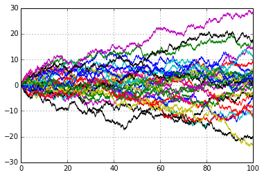
In the picture below you will see \(180\) sample paths of simulated random walks, across \(100\) ticks of unit time. The picture is cone shaped and you will notice that that paths are quite densely packed around zero (the expected value) and their endpoints thin out a little beyond \(\pm 10\) (\(10=\sqrt{100}\) being the standard deviation of the final destination).

There are a few things we can play with here. The first is to notice that we have been dealing with a so-called symmetric random walk, where the probability of a \(+1\) jump is the same as that of a \(-1\) fall. If we drop this requirement and essentially let an unfair (weighted) coin determine the up or down step then we are really dealing with a random variables of the form

\[ X_{i}=\begin{cases} +1\quad {\rm{with}}\,\,{\rm{probability}}\,\,=p;\\ -1\quad {\rm{with}}\,\,{\rm{probability}}\,\,=q, \end{cases} \]

where \(p,q\in [0,1]\) and \(p+q=1.\) Let’s repeat the calculations above for this general version of the random walk. First we notice that

\[ \begin{aligned} \mathbb{E}[X_{i}]&=1\times \mathbb{P}[X_{i}=1]+(-1)\times \mathbb{P}[X_{i}=-1]\\ &= 1\times p-1\times q\\ &= p-q\\ &=2p-1, \end{aligned} \]

and this leads to a new expected final value:

\[ \mathbb{E}[W^{(1)}(n)]=\mathbb{E}\Bigl[\sum_{i=1}^{n}X_{i}\Bigr]=\sum_{i=1}^{n}\mathbb{E}[X_{i}]=n(2p-1). \]

Similarly, for variance of the up/down step random variable, we have

\[ \begin{aligned} {\mathrm{var}}[X_{i}]&=\mathbb{E}[X_{i}^{2}]-\mathbb{E}[X_{i}]^{2}\\ &=(1)^{2}\times \mathbb{P}[X_{i}=1]+(-1)^{2}\times \mathbb{P}[X_{i}=-1]-(2p-1)^{2}\\ &= p+q-(2p-1)^{2}\\ &= 1-(2p-1)^{2}\\ &=2p\times(2-2p)=4p(1-p)=4pq, \end{aligned} \]

and this leads to the variance of the endpoint of the new random walk being

\[ \begin{aligned} {\mathrm{var}}\left(W^{(1)}(n)\right)&={\mathrm{var}}\left(\sum_{i=1}^{n}X_{i}\right)=\sum_{i=1}^{n}{\mathrm{var}}(X_{i})=4pqn= 4np(1-p). \end{aligned} \]

The picture below gives an example of a random walk with \(p=0.6\) and \(q=0.4,\) you can see in this snapshot that there is more of a prevalence to move up than down, as you would expect with these probabilities.

More interestingly perhaps is the next picture which, as before, shows \(180\) sample paths of simulated random walks, across \(100\) ticks of unit time. The picture remains cone shaped except, this time rather than bunching around zero these paths are quite densely packed around the black line (the expected value line given by \((p-q)t= (0.6-0.4)t=0.2t\)). The expected endpoints of the paths is \(20=0.2\times 100\) and the final landing points once more thin out a little beyond \(\pm 10\) this is not surprising as the standard deviation of the final destination is given by \(\sqrt{4\times 100\times 0.6\times 0.4}=\sqrt{96}\approx 9.798.\)

Note that it is straightforward to show, with a little bit of calculus, that the maximum variance of this general random walk occurs in the symmetric version when \(p=\frac{1}{2}.\)

SPaths of an asymmetric random walk

The next thing we can play around with is to allow more than one step to occur across each tick of unit time or we could reduce the size of the step.

\(\diamond\) If we now allow a change to the rules of the model and say, at each tick of unit time we will allow \(k\) steps to occur.

\(\diamond\) An alternative way to view the above is to stick with taking one step but reducing the tick of unit time from \(1\) to \(\frac{1}{k}.\)

What we are doing here is experimenting with a finer and finer random walk, although we need to be careful that we keep the nice cone shape of paths, i.e.,
the position of the walker does not explode far far away from the starting point. Statistically speaking, at any point in time we want the variance to remain constant, even if we allow many many more steps per unit time. Lets see what happens if we just barge into this without much thought.

The image on the top of the picture you see below shows \(20\) typical paths when we run the random walk with the following the change of rule:

\(\diamond\) the unit step size stays the same but we now squeeze TEN of them (up or down) into a single tick of time (equivalently a full step is now take every \(\frac{1}{10}\) of a time tick).

\(\diamond\) We note that the lower image is the one we have already encountered, where only one step is taken in the time tick.

At first glance of the upper image, the paths do not look so different from those we have already encountered (lower image), they appear less jagged but this is just because we have so many more points, \(1000\) for the top image v \(100\) for the bottom image. The more serious difference becomes apparent when we look at just how far we are moving; in the lower image we are able to keep the path confined to a cone shape, but if we superimposed this ‘cone’ onto the top picture then the see that the path quite quickly break free of it; after just \(20\) time ticks there are paths that are almost \(40\) steps away from their starting position! (this doesn’t happen in the entire across the whole \(100\) time ticks when just one step per tick is allowed)

Mathematically, this is not surprising the variance of the final position is the same as the total number of steps taken, so by squeezing \(10\) more steps across each time tick the variance is ten times bigger at any given time step. Under the original rules we know that in the first time tick we will only be one step away from where we started, under the new rule we could (potentially) be ten steps away.

If we want to design a walk with more than one step per time tick but that doesn’t blow up like this then, quite simply, we have to shorted the distance of our steps. Let’s remind ourselves of the issue

\(\bullet\) Suppose it takes \(n\) ticks of unit time until we are at the future time \(T\) on our random walk.

1. If we allow one symmetric random unit step every time tick then the variance of our final position \(W^{(1)}(T)\) is

\[ \begin{aligned} {\mathrm{var}}\left(W^{(1)}(T)\right)&={\mathrm{var}}\left(\sum_{i=1}^{T=n}X_{i}\right)=\sum_{i=1}^{T=n}{\mathrm{var}}(X_{i})=n=T. \end{aligned}\tag{3.5} \]

2. If we now allow \(k\) symmetric random unit steps every time tick then the variance of our final position \(W^{(k)}(T)\) (after \(k\times n\) steps) is

\[ \begin{aligned} {\mathrm{var}}\left(W^{(k)}(T)\right)&={\mathrm{var}}\left(\sum_{i=1}^{T=kn}X_{i}\right)=\sum_{i=1}^{T=kn}{\mathrm{var}}(X_{i})=kn=kT. \end{aligned} \]

We don’t want the variance to change so the plan to is to shorten the step. Recall that variance of a random variable \(Z\) say, scales like

\[ {\mathrm{var}}\left(\epsilon Z\right)=\epsilon^{2}{\mathrm{var}}\left( Z\right) %\quad{\rm{equivalently}}\,\,\,\,{\mathrm{var}}\left(\frac{ %Z}{\lambda}\right)=\frac{1}{\lambda^{2}}{\mathrm{var}}\left( Z\right)\quad \epsilon >0. \]

Let us reduce the step size of our walk by a factor \(0<\epsilon<1,\) this means we allow \(k\) symmetric random steps every time tick but now the size of each step can either be up or down by a small amount \(\epsilon.\) Thus, every \(\frac{1}{k}\) of a standard tick of unit time, the random variable that describes our potential move is given by

\[ Y_{i}=\epsilon X_{i}=\begin{cases} +\epsilon\quad {\rm{with}}\,\,{\rm{probability}}\,\,=\frac{1}{2};\\ -\epsilon\quad {\rm{with}}\,\,{\rm{probability}}\,\,=\frac{1}{2}. \end{cases} \]

Then the new variance of the final position \(W^{(k,\epsilon)}(T)\) is

\[ \begin{aligned} {\mathrm{var}}\left(W^{(k,\epsilon)}(T)\right)&={\mathrm{var}}\left(\sum_{i=1}^{T=kn}Y_{i}\right)\\ &=\sum_{i=1}^{T=kn}{\mathrm{var}}(Y_{i})\\ &=\sum_{i=1}^{T=kn}{\mathrm{var}}(\epsilon X_{i})\\&=\epsilon^{2}\sum_{i=1}^{T=kn}{\mathrm{var}}(X_{i})=\epsilon^{2}kn=\epsilon^{2}kT. \end{aligned} \tag{3.6} \]

We can see immediately now that, by comparing (3.5) and (3.6), we are able to match the variance of the original random walk to that of the scaled and more frequent version by setting \(\epsilon =\frac{1}{\sqrt{k}}.\) The lesson we learn from all of this is:

\(\bullet\) If we want increase the frequency of steps per unit time from \(1\) (in the standard case) to \(k\) in our random walk while retaining the same properties then we must reduce the size of each step by a factor of \(\frac{1}{\sqrt{k}};\) so there is a link between frequency of steps and size of steps.

\(\bullet\) An alternative, and possibly easier, way of thinking about this is that if we change the rules so that instead of the standard one unit step for every tick of unit time we now allow a step across a shorter interval of time \(\delta t (=\frac{1}{k})\) say, then in order to ensure the new walk has the same statistical features as the standard one, we must scale the step size down by a factor of \(\sqrt{\delta t}\,\, (=\frac{1}{\sqrt{k}}).\)

The picture below show reassures us that this scaling in both time and distance really is exactly what is needed, the image on the top shows \(30\) paths where the frequency of steps has been increased by a factor of \(10,\) AND the length of the steps has been reduced by a factor of \(\frac{1}{\sqrt{10}}.\) The lower image is the standard, and by now familiar, symmetric random walk.

Paths of the random walk scaled in time and distance

Paths of the standard symmetric random walk

A few things to notice:

\(\bullet\) Independent increments: for \(0<t_{1}<t_{2}<t_{3}<t_{4},\) we look at the two increments, the first one over \((t_{1},t_{2})\) i.e.,
\(W^{(k)}(t_{2})- W^{(k)}(t_{1})\) and the second over \((t_{3},t_{4}),\) i.e., \(W^{(k)}(t_{4})- W^{(k)}(t_{3}),\) these are independent.

\(\bullet\) As we have already established the expected value of the time-and-distance scaled random walk is zero \(\mathbb{E}[W^{(k)}(t)]=0\) and variance is proportional to the time interval \({\rm{var}}(W^{(k)}(t))=t.\)

\(\bullet\) Using the central limit theorem as \(n = kt\) grows large \(W^{(k)}(t),\) being a large sum of i.i.d. random variables, is well approximated by a normal random variable with the mean and variance quoted above.

If we look back at the definition of Brownian motion you will see that the random walk we have constructed is almost there, the only thing that is missing is that we haven’t got and that is continuity and the precision on the normal random approximation; the full strength version of the central limit theorem is precisely what we need here because Brownian motion emerges when we stop speaking about allowing \(n\) and \(k\) to be large, under the constraint that \(n=kt\) and to take the limit as \(n\) and \(k\) tend to \(\infty,\) or, equivalently to let the interval \(\delta t\) across which we can have a step of size \(\frac{1}{\sqrt{\delta t}}\) to approach zero. Upon taking this limit we arrive at Brownian motion, precisely as in our definition. We write

\[ W_{t}=\lim_{k\to \infty}W^{(k,\frac{1}{\sqrt{k}})}(t),\quad {\rm{or}}\,\,\,{\rm{equivalently}}\,\,\, W_{t}=\lim_{\delta t\to 0}W^{(\frac{1}{\delta t},\sqrt{\delta t})}(t), \]

If you are interested in a much more substantial investigation of how Brownian motion arises as the limit of the scaled-in-space-and-time random walk then you can consult the first chapter of Kwok’s book, We note in passing the we that it is in honour of Wiener’s work that we use the letter \(W\) to denote a Brownian motion.

Before we move back to the modeling framework we have developed let us pause to accomplish some calculations using Brownian motion.

Example 3.1 (Brownian Motion Calculations) With standard Brownian motion \(W_{t}\) always keep in mind the simple fact that \(W_{t}\sim N(0,t)\) and so \(\frac{1}{\sqrt{t}}W_{t}\sim N(0,1)\) (we have tables of values for the standard normal distribution - if we are far from a software package).

\(\bullet\) VERY EASY: What is \(\mathbb{P}[W_{3}<0]?\) This is easily computed as follows

\[ \mathbb{P}[W_{3}<0]= \mathbb{P}\Bigl[\frac{1}{\sqrt{3}}Z<0\Bigr]=\mathbb{P}\Bigl[Z<0\Bigr]=\Phi(0) = \frac{1}{2}. \]

\(\bullet\) EASY: What is \(\mathbb{P}[W_{100}<W_{80}]?\) This use the fact that the increments of a Brownian motion are also normally distributed, i.e., that for \(0<s<t\) \(W_{t}-W_{s}\sim N(0,t-s).\) This allows us to deliver the answer to this question as follows:

\[ \mathbb{P}[W_{100}<W_{80}]=\mathbb{P}[W_{100}-W_{80}<0]=\mathbb{P}\Bigl[\frac{W_{100}-W_{80}}{\sqrt{100-80}}<0\Bigr]=\mathbb{P}\Bigl[Z<0\Bigr]=\Phi(0) = \frac{1}{2}. \]

\(\bullet\) RELATIVELY EASY: What is [W_{100}<W_{80}+2]?$ Applying the same logic as above we arrive that the answer:

\[ \begin{aligned} \mathbb{P}[W_{100}<W_{80}+2]=\mathbb{P}[W_{100}-W_{80}<2]&=\mathbb{P}\Bigl[\frac{W_{100}-W_{80}}{\sqrt{100-80}}<\frac{2}{\sqrt{100-80}}\Bigr]\\ &=\mathbb{P}\Bigl[Z<\frac{2}{\sqrt{20}}\Bigr]=\\ &=\Phi\left(\frac{2}{\sqrt{20}}\right) \approx 0.67. \end{aligned} \]

\(\bullet\) A LITTLE HARDER: What is \(\mathbb{P}[W_{3}<W_{2}+2, \,\,{\rm{and}}\,\, W_{1}<0 ]?\) Here we want the probabilities of two events that are independent of each other. So this just means we have to calculate both probabilities and then multiply them together. Here it goes:

\[ \begin{aligned} \mathbb{P}[W_{3}<W_{2}+2, \,\,{\rm{and}}\,\, W_{1}<0 ]&=\mathbb{P}[W_{3}<W_{2}+2, \,\,{\rm{and}}\,\, W_{1}-W_{0}<0 ]\\ &=\mathbb{P}[W_{3}-W_{2}<2]\mathbb{P}[W_{1}-W_{0}<0]\\ &=\mathbb{P}[Z<2]\mathbb{P}[Z<0]\\ &=\Phi(2)\Phi(0)\\&= \frac{\Phi(2)}{2}. \end{aligned} \] \(\bullet\) SEEMINGLY IMPOSSIBLE: What is \(\mathbb{P}[W_{3}<2, \,\,{\rm{and}}\,\, W_{4}<3 ]?\) Here the difficulty is that te two events are not independent, the first event concerns the interval \((0,3)\) and the second one concerns the interval \((0,4)\) - these two overlap and there is no way to progress using the approaches we have used so far. In order to solve this problem we would need additional information on the measure of covariance or correlation between the two events.

The Brownian motion that we have been working with is often referred to as the standard Brownian motion. Given that Brownian motion was discovered in the context of examining the random diffusion of particles it should not surprise you that the standard model can be extended so that it can be adapt to allow for a non-zero drift rate \(\mu\) and a diffusion coefficient \(\sigma.\) We have the following more general definition:

Definition 3.2 (Brownian Motion with Drift and Diffusion) A Brownian motion with drift rate \(\mu\) and diffusion coefficient \(\sigma>0\) is a stochastic process \(\{B_{t}:t\ge 0\}\) that satisfies the following properties

1. \(B_{0}=0\) and the sample paths of \(B_{t}\) are continuous.

2. Every increment \(B_{t}-B_{s}\) is \(N(\mu (t-s),\sigma^{2}(t-s))\) for all \(t\ge s\ge 0.\)

3. For every partition of time \(0<t_{1}<t_{2}<\cdots <t_{n}\) the increments \(B_{t_{1}}, B_{t_{2}}-B_{t_{1}},\ldots,B_{t_{n}}-B_{t_{n-1}}\) are independent (independent increments) and, in view of \(2\) above, \(B_{t_{k}}-B_{t_{k-1}}\sim N(\mu (t_{k}-t_{k-1}),\sigma^{2}(t_{k}-t_{k-1})).\)

A nice shorthand way of expressing this more general Brownian motion is to write in terms of the standard version that we know very well, specifically a Brownian motion \(B_{t}\) with drift \(\mu\) and diffusion \(\sigma>0\) is given by

\[ B_{t}=\mu t+ \sigma W_{t}. \]

3.2.2 Properties of Brownian Motion

Now that we understand some of the mathematical background of the Brownian motion, in terms of how it emerges from the random walk, we will now pick out some of its fascinating (sometime they are!) properties.

1. We acknowledge that the Brownian motion is a continuous function of time. Now the mathematician in you may wonder what its derivative is? Well, you are in for a shock. Brownian motion, although continuous, is not differentiable anywhere. To see this we go back to first principles, for a nicely behaved function of time \(f(t)\) say, we would compute its derivative formally in two steps

\(\bullet\) First, for a small time increment \(\delta t\) we consider the local rate of chance given by

\[ \frac{f(t+\delta t)-f(t)}{\delta t}. \]

\(\bullet\) Second, we take the limit of the local rate as \(\delta t \to 0\) in order to get the instantaneous rate of change \(f^{\prime}(t)\) i.e., we consider the local rate of change given by

\[f^{\prime}(t)=\lim_{\delta t \to 0} \frac{f(t+\delta t)-f(t)}{\delta t}. \]

Now if we do the same for Brownian motion the local rate of change is a normal random variable with an enormous variance (since \(\delta t\) is small)

\[ \frac{W_{t+\delta t}-W_{t}}{\delta t} \sim N(0,\frac{1}{\delta t}), \]

clearly this blows up as \(\delta t \to 0.\) An alternative way of convincing yourself of this is to use the fact that the increment on the numerator \(W_{t+\delta t}-W_{t}\) has the distribution \(N(0,\delta t)\) and thus we can write the local rate of change as

\[ \frac{W_{t+\delta t}-W_{t}}{\delta t} = \frac{\sqrt{\delta t}\epsilon}{\delta t}=\frac{\epsilon}{\sqrt{\delta t}}\quad {\rm{where}}\,\,\, \epsilon \sim N(0,1), \]

and clearly this becomes infinite as \(\delta t \to 0.\)

2. Although Brownian motion is continuous in time it is not possible to capture it in a free hand sketch or plot, this is because it has a fractal nature to it; in simple terms this means it has the self-similarity property; you notice that even it exhibits the same wiggly path at all levels of magnification, this explains why it isn’t possible to take the derivative because, even at very tiny time intervals there is a wiggly path across it (recall - for the nice functions we deal with in calculus the more you zoom in on the curve the more it resembles a straight line - not so with Brownian motion!) The picture below shows this fractal feature off quite nicely.

3. The next couple of insights does involve me introducing TWO new properties. Now, I perfectly understand that when you are studying a non-trivial topic (such as we are doing now with Brownian motion) then the last thing you need is for new concepts to be dragged into the story; it can feel overwhelming. However, rest assured despite the formal definitions you are about to read I do hope that I can convey how these fit in to what we are doing, there is certainly no need whatsoever for you to head off on a journey to find out more details than I give here (unless of course you simply want to). Here’s the first:

Definition 3.3 (The Markov Property) A stochastic process \(X_{t}\) has the Markov property if, given the value \(X_{s}\) at some time \(s>0,\) the future value \(X_{t}\) at some time \(t>s\) depends only on the value \(X_{s},\) it does not depend on any of the previous values of the process in the time beforehand, i.e., those values \(X_{\tau}\) for \(0<\tau<s.\)

To unpick the formal definition it basically means that if we pause time on our random process (at time \(s\)) and wonder where it is going to head next, then we can be sure that no matter how well we examine the path so far it will not inform us of where we are going next; all that we know is that we are moving on from the current position. If you think of this from a financial point of view it begins to make sense. We’ve all heard those taglines on adverts for investment products on offer at our local banks ‘past performance is no guarantee of future success’ (or something along those lines). This is precisely the layman’s version of saying that the investment has the Markov property. So you won’t be surprised to hear that Brownian motion has this property, this can easily be seen from its definition, note that the intervals \((0,\tau)\) and \((s,t)\) are non-overlapping whenever \(\tau <s\) and so the increments

\[ W_{\tau}=W_{\tau}-W_{0}\quad {\rm{and}}\quad W_{t}-W_{s} \]

are independent, meaning that knowledge of \(W_{\tau}\) for \(\tau <s\) has no effect on the distribution of \(W_{t}-W_{s},\) this is precisely the Markov property for Brownian motion.

To help you out from a more mathematical perspective let’s try and capture the Markov property in a single useful equation. What we will do, once again is pause time as \(t\) say, and imagine that we have access to the history of how the stochastic process has evolved so far, i.e., we are armed with the information set \(\{X_{\tau}:0\le\tau\le t\}\) from this moment in time and given all of the information we have we want to compute the expected future value at time \(t+h\) where \(h>0.\) Given that we have information available this is not the ordinary expected value of \(X_{t+h}\) it is what we call a conditional expectation i.e., what is expectation viewed from time \(t\) of the future under the condition that we already know the path so far. Mathematically we write this as

\[ \mathbb{E}[X_{t+h}|\,\,X_{\tau}\,\,\,\,\ {\rm{for}}\,\, 0\le\tau\le t\,\,] \]

and we say, the expected value of \(X_{t+\tau}\) given the history of the process up to an including time \(t.\) You will also very frequently see this written in the following shorter version

\[ \mathbb{E}_{t}[X_{t+h}] \]

where the subscript \(t\) on the expectation operator signifies that, in taking the expectation, we are using all information we have on the path up until time \(t.\)

Now, if the stochastic process has the Markov property then we know that the past history of the process has no influence on the future value - all we know is that we’ll be moving on from the current point \(X_{t},\) thus we can see that if \(X_{t}\) has the Markov property we can slice away the past history from the information set and write

\[ \mathbb{E}[X_{t+h}|\,\,X_{\tau}\,\,\,\,\ {\rm{for}}\,\, 0\le\tau\le t\}]=\mathbb{E}[X_{t+h}|\,\,X_{t}\,]\tag{3.7} \]

which is much neater.

OK, we are done with the Markov property - we have established that Brownian motion has it, that its essence is captured in the (eq:mark), that it makes sense in a financial context and I’m fairly confident that is all we will ever need. DONE!

The second property also has a fancy name and focuses on the computation of the conditional expectation mentioned above. Here it is:

Definition 3.4 (The Martingale Property) A stochastic process \(X_{t}\) has the Martingale property (or. more commonly. is a martingale), if

1. \(\mathbb{E}[|X_{t}|]<\infty\)

2. \(\mathbb{E}[X_{t+h}\,\,|\,\,X_{\tau}\,\,\,\,\ {\rm{for}}\,\, 0\le\tau\le t\,\,]=X_{t}\)

Unpicking this we can say that our stochastic process is a martingale and we pause it at some time \(t,\) then the best prediction of all future values is simply its current (paused) value \(X_{t}.\) Obviously, if the process is a martingale AND has the Markov property then property \(2\) above collapses to

\[ \mathbb{E}[X_{t+h}\,\,|\,\,X_{t}\,\,]=X_{t},\quad {\rm{or}}\,\,{\rm{equivalently}}\quad \mathbb{E}_{t}[X_{t+h}]=X_{t}. \]

It is reasonably straightforward to show that Brownian motion is a martingale. In order to show it we must establish that

\[\mathbb{E}_{t}[W_{t+h}]=W_{t},\quad {\rm{for}}\,\,h>0. \]

To see it we write

\[ W_{t+h}=W_{t+h}-W_{t}+W_{t}=\left(W_{t+h}-W_{t}\right)+W_{t} \]

We recognise the term in the bracket as an increment of Brownian motion over the future time interval \((t,t+h)\) we know its outcome to be independent from the earlier non-overlapping time interval \((0,t).\) Furthermore, as an increment of Brownian motion we know it is \(N(0,h).\) Using this insight we can achieve our goal as

\[ \begin{aligned} \mathbb{E}_{t}[W_{t+h}]&=\mathbb{E}_{t}[\left(W_{t+h}-W_{t}\right)+W_{t}]\\ &=\mathbb{E}_{t}[\left(W_{t+h}-W_{t}\right)]+\mathbb{E}_{t}[W_{t}]\\ &=\mathbb{E}[\left(W_{t+h}-W_{t}\right)]+W_{t}\\ &=0+W_{t}=W_{t} \end{aligned} \]

4. The next thing we will look at is the differential equation satisfied by a Brownian motion. We will start off easy, recall that the Brownian motion with a constant drift \(\mu\) and a diffusion coefficient \(\sigma\) can be written as

\[ B_{t}=\mu t +\sigma W_{t}. \]

Quite trivially, it is easy to see that this Brownian motion is the solution to:

\[ dB_{t}=\mu dt +\sigma dW_{t}. \]

What we have above is an example of a stochastic differential equation and the new aspect to it, as far as we are concerned is the term \(dW_{t}.\) We’ve already established that (standard) Brownian motion is pretty weird, fractal, continuous but nowhere differentiable… So how do we make sense of a term like \(dW_{t}\) an infinitesimally small increment of Brownian motion. Well, to do this properly would take us too far off track and so here I will simply provide an intuitive guide. We begin by letting \(\delta W_{t}\) denote the change in \(W_{t}\) during the time interval \(t\to t+\delta t,\) then using the second property of the definition we have that

\[ \delta W_{t} = W_{t+\delta t}-W_{t}\sim N(0,\delta t)\implies \delta W_{t} = Z_{t} \sqrt{\delta t},\,\,\,{\rm{where}}\,\,\,Z_{t}\sim N(0,1). \]

In the differential limit as \(\delta t \to 0\) we get the continuous version of incremental model which we write as

\[ dW_{t}=Z_{t}\sqrt{dt}, \quad Z_{t}\sim N(0,1). \tag{3.8} \]

We can see immediately from (3.8) that

\[ \mathbb{E}[dW_{t}]=0 \quad{\rm{and}}\quad var(dW_{t})=dt \]

Similarly we are also able to deduce that, for the scaled differential increment \(dtdW_{t}\) we have

\[ \mathbb{E}[dtdW_{t}]=0 \quad{\rm{and}}\quad var(dtdW_{t})=(dt)^{3} \]

Finally, if we investigate the behaviour of \(dW_{t}^{2}\) in the same way we find

\[ \mathbb{E}[dW_{t}^{2}]=\mathbb{E}[dt Z_{t}^{2}]= dt\mathbb{E}[ Z_{t}^{2}]=dt \]

and

\[ \begin{aligned} var(dW_{t}^{2})&=\mathbb{E}[dW_{t}^{4}]-\left(\mathbb{E}[ dW_{t}^{2}]\right)^{2}\\&=\mathbb{E}[(dt)^{2}Z_{t}^{4}]-\left(\mathbb{E}[ dtZ_{t}^{2}]\right)^{2}\\ &= (dt)^{2}(3-1)=2(dt)^{2} \end{aligned} \]

Recall our rule that if a small time interval is raised to a power that is greater than one then we will consider it to be zero as it is so negligibly small. Well applying this rule above leads us to contemplate that both \(dW_{t}^{2}\) and \(dtdW_{t}\) have zero variance. But a variable with zero variance is not random and so its expected value is really its actual value. Thus, for this case we conclude that

\[ dW_{t}^{2}=dt \quad {\rm{and}}\quad dtdW_{t} =0. \tag{3.9} \]

These discoveries encapsulated above (3.9) are commonly referred to as the It\(\hat{{\rm{o}}}\) rules of stochastic calculus; these are named after Kiyoshi It\(\hat{{\rm{o}}}\) (1915-2008) the Japanese mathematician who pioneered the theory of stochastic differential equations; this area of study is commonly referred to as It\(\hat{{\rm{o}}}\) calculus.

5. So that you don’t feel short-changed I will present here the cast-iron proof of the first It\(\hat{{\rm{o}}}\) rule, i.e., that \(dW_{t}^{2}=dt\). The proof revolves around the calculation of the so-called quadratic variation of Brownian motion over a certain time interval \([0,T].\) In case you have not encountered this notion before let’s suppose we have any old function \(f(t)\) defined on \([0,T].\) There are three steps involved:

\(\bullet\) First we make a partition \(\Pi\) of the interval \([0,T]\) of the form

\[ 0=t_{0}<t_{1}<\cdots <t_{N}=T \]

We measure how ‘fine’ the partition is by the width of the largest gap between two successive points, i.e., we define

\[ \Delta = \max \{|t_{k+1}-t_{k}|:k=0,1,\ldots,N-1\} \]

\(\bullet\) Second we compute the quadratic variation corresponding to our partition we define this as

\[ Q_{\Pi}= \sum_{k=0}^{N-1}\left(f(t_{k+1})-f(t_k)\right)^{2} \]

\(\bullet\) Third we consider the limit of the quantity \(Q_{\Pi}\) as the quantity \(\Delta \to 0,\) i.e., as the partitions get finer what is the limiting value of \(Q_{\Pi}.\)

We will employ the equally spaced partition, specifically, if we are using \(N+1\) points then we set \(\Delta = \frac{T}{n}\) and define \(t_{k}=kh,\) for \(k=0,1,\ldots, N.\) We’ll write the quadratic variation of the standard Brownian motion as

\[ Q_{N}=\sum_{k=0}^{N-1}\left(W_{(k+1)h}-W_{kh}\right)^{2} \]

OK, in the brackets we have independent increments of Brownian motion, each one being a \(N(0,h)\) random variable. This means we can write

\[ Q_{N}=\sum_{k=0}^{N-1}\left(W_{(k+1)h}-W_{kh}\right)^{2} \] \[ Q_{N}=\sum_{k=0}^{N-1}\left(\sqrt{h}Z_{k}\right)^{2}=h\sum_{k=0}^{N-1}Z_{k}^{2}\quad {\rm{where}} \,\,\,\,Z_{k}\sim N(0,1) \,\,\, (i.i.d). \]

Immediately we can work compute the expected value of \(Q_{N}:\)

\[ \mathbb{E}[Q_{N}]=\mathbb{E}\Bigl[h\sum_{k=0}^{N-1}Z_{k}^{2}\Bigr]=h\sum_{k=0}^{N-1}\mathbb{E}[Z_{k}^{2}]=h\sum_{k=0}^{N-1}1=hN=T, \]

we note that this is independent of \(N\).

Next we compute the variance of \(Q_{N}:\)

\[ \begin{aligned} {\rm{var}}(Q_{N})={\rm{var}}\Bigl(h\sum_{k=0}^{N-1}Z_{k}^{2}\Bigr) &= \sum_{k=0}^{N-1}{\rm{var}}(hZ_{k}^{2})\\ &=h^{2}\sum_{k=0}^{N-1}{\rm{var}}(Z_{k}^{2})\\ &=h^{2}\sum_{k=0}^{N-1}\left(\mathbb{E}[Z_{k}^{4}]-\left(\mathbb{E}[Z_{k}^{2}]\right)^{2}\right)\\ &=h^{2}\sum_{k=0}^{N-1}(3-1)\\ &=2h^{2}N=\frac{2(hN)^{2}}{N}=\frac{2T^{2}}{N}. \end{aligned} \]

What we notice here is that as \(N\to \infty\) the variance vanishes, this means that the the limit of quadratic variation is time \(T.\)

We note that if we take the plain variation, dropping the squares, we have the sum of independent increments

\[ \sum_{k=0}^{N-1}\left(W_{(k+1)h}-W_{kh}\right) = \underline{W_{h}}-W_{0}+\underline{W_{2h}}-\underline{W_{h}}+W_{3h}-\underline{W_{2h}}+\cdots +W_{Nh}-W_{(N-1)h} \]

A careful glance shows that we have what is known as a telescoping sum where the positive term of one increment is canceled by the negative term from the next. In the end we see

\[ W_{T}= W_{T}-W_{0}=\sum_{k=0}^{N-1}\left(W_{(k+1)h}-W_{kh}\right) \]

this is independent of \(N\) and so taking the limit as \(N\to \infty\) we can pass from finite sums of increments to the integral of the differential element of Brownian motion, i.e., we conclude that

\[ W_{T}=\int_{\tau=0}^{T}dW_{\tau}, \]

or more generally we can express the Brownian motion as the stochastic integral

\[ W_{t}=\int_{\tau=0}^{t}dW_{\tau}. \]

Arguing in precisely the same way for the quadratic variation we arrive at

\[ T=\int_{0}^{T}(dW_{t})^{2}. \]

But, in this case, we can also reach the same conclusion using the deterministic integral

\[ T= \int_{0}^{T}dt. \]

This leads us to the cast-iron conclusion that \((dW_{t})^{2}=dt.\)

3.2.3 A Sample of It\(\hat{{\rm{o}}}\) Calculus

We have seen that a general Brownian motion with drift rate \(\mu\) and diffusion coefficient \(\sigma>0\) is expressed as

\[ B_{t}=\mu t +\sigma W_{t} \]

if we consider the obvious stochastic differential equation

\[ dB_{t}=\mu dt +\sigma dW_{t}, \tag{3.10} \]

then it is not controversial to conclude that our Brownian motion process is a solution to (3.10). More interesting (and also more challenging) is to allow the drift and diffusion terms to be deterministic functions of the underlying process and so we turn our attention (albeit very briefly) to stochastic differential equations of the form

\[ dx_{t}=\mu(x_{t},t) dt +\sigma(x_{t},t) dW_{t}, \tag{3.11} \]

Such a differential equation is often referred to as the random walk for the process the It\(\hat{{\rm{o}}}\) process \(x_{t}.\) Note that without the \(dW_{t}\) term we would be left with a familiar ordinary differential equation of the form

\[ \frac{dx_{t}}{dt}= \mu(x_{t},t) \]

which, if we know the initial condition \(x_{0},\) we could solve by integration,

\[ x_{t}-x_{0}= \int_{s=0}^{t}dx_{s} = \int_{s=0}^{t}\mu(x_{s},s)ds \implies x_{t} =x_{0}+ \int_{s=0}^{t}\mu(x_{s},s)ds. \]

The obvious approach is to emulate the integration route in the stochastic setting BUT we are now dealing with something brand new - the term

\[ \int_{s=0}^{t}\sigma(x_{s},s)dW_{s}. \tag{3.12} \]

we already know some crazy features of the standard Brownian motion \(W_{t}\), it is not differentiable and has a fractal nature, so how can we be sure that integrating a function against it, as in (3.12), is well defined. It turns out that, within the study of It\(\hat{{\rm{o}}}\) calculus, it is possible to identify some technical conditions that ensure this integral is well-defined. Thankfully, for everything that we encounter in this course, these conditions are always satisfied. This sounds like great news but even though we know these integrals exist, we still have to calculate them and this is not always a straight forward task. However, we really do have a lot to give thanks for because there is a quicker way which relies on a real game-changer of a result that is commonly referred to as It\(\hat{{\bf{o}}}\)’s Lemma.

It\(\hat{{\bf{o}}}\)’s Lemma is motivated by the following. We have in our possession a process \(x_{t}\) whose random walk is given by (3.11). Next we are supplied with a function \(f(x,t)\) which is differentiable with respect to the time variable \(t\) and is (at least) twice differentiable with respect to the space variable \(x.\) We use this function to create a new process

\[ y_{t}=f(x_{t},t). \]

The question is… what is the random walk for this new process \(y_{t}\)?

It\(\hat{{\bf{o}}}\)’s Lemma provides the answer. I will now show how we get to it but in doing so you must accept if, in the course of our investigation, we ever encounter terms involving powers of \(dt\) that are bigger than one then we ignore them. I’ve mentioned this before, the simple argument being that \(dt\) is already infinitesimally small so raising it to a ‘higher’ power makes it smaller still - so we neglect it. With this rule of established we employ a second order Taylor approximation to write:

\[ dy_{t}=df(x_{t},t)=\frac{\partial f}{\partial x}dx_{t}+\frac{\partial f}{\partial t}dt+\frac{1}{2}\frac{\partial^{2} f}{\partial x^{2}}(dx_{t})^{2}. \tag{3.13} \]

You may wonder why I am so confident to be able to truncate at the second spacial derivative, well here’s where our It\(\hat{{\bf{o}}}\) rules come to our rescue. We know the random walk for \(x_{t}\) is given by

\[ dx_{t}=\mu(x_{t},t) dt +\sigma(x_{t},t) dW_{t}, \]

so squaring this gives us the term given by

\[ \begin{aligned} (dx_{t})^{2} &=\left(\mu(x_{t},t) dt +\sigma(x_{t},t) dW_{t}\right)^{2}\\ &=\mu(x_{t},t)^{2} \underline{(dt)^{2}}+\mu(x_{t},t)\sigma(x_{t},t) \underline{dtdW_{t}}+\sigma(x_{t},t)^{2}\underline{(dW_{t})^{2}} \end{aligned} \]

Consider the terms that are underlined. The first one sees us squaring \(dt,\) and, adhering to our powers-of\(dt\)-rule, we can immediately ignore. The other two terms are dealt with by the It\(\hat{{\bf{o}}}\) rules (3.9), \(dtdW_{t}=0\) and \(dW_{t}^{2}=dt,\) and so this collapses to

\[ (dx_{t})^{2}=\sigma(x_{t},t)^{2}dt \tag{3.14} \]

and so plugging this into @ref{sectay}, together with the known random walk for \(x_{t},\) we arrive at

\[ \begin{aligned} dy_{t}=df(x_{t},t)&=\frac{\partial f}{\partial x}dx_{t}+\frac{\partial f}{\partial t}dt+\frac{1}{2}\frac{\partial^{2} f}{\partial x^{2}}(dx_{t})^{2}\\ &=\frac{\partial f}{\partial x}\left(\mu(x_{t},t) dt +\sigma(x_{t},t) dW_{t}\right)+ \frac{\partial f}{\partial t}dt+\frac{1}{2}\frac{\partial^{2} f}{\partial x^{2}}\sigma(x_{t},t)^{2}dt\\ &=\Bigl(\mu(x_{t},t)\frac{\partial f}{\partial x}+\frac{\sigma(x_{t},t)^{2}}{2}\frac{\partial^{2} f}{\partial x^{2}}+\frac{\partial f}{\partial t}\Bigr)dt+ \Bigl(\sigma(x_{t},t)\frac{\partial f}{\partial x}\Bigr)dW_{t}. \end{aligned} \]

This development is the famous It\(\hat{{\rm{o}}}\)’s Lemma, we’ve proved it! So famous and important, in fact that we should probably state it. It’s a big deal!

Lemma 3.1 (Itos Lemma) Let \(x_{t}\) be an It\(\hat{{\rm{o}}}\) process, i.e., a stochastic process that satisfies

\[ dx_{t}=\mu(x_{t},t) dt +\sigma(x_{t},t) dW_{t}, \]

where \(\mu(x,t)\) is a (local) deterministic drift function and \(\sigma(x_{t},t)\) s a (local) deterministic diffusion function. Let \(f(x,t)\) be a function that is differentiable with respect to the time variable \(t\) and is (at least) twice differentiable with respect to the space variable \(x.\) Then \(y_{t}=f(x,t)\) is an It\(\hat{{\rm{o}}}\) process that satisfies

\[ dy_{t}=df(x_{t},t)=\Bigl(\mu(x_{t},t)\frac{\partial f}{\partial x}+\frac{\sigma(x_{t},t)^{2}}{2}\frac{\partial^{2} f}{\partial x^{2}}+\frac{\partial f}{\partial t}\Bigr)dt+ \Bigl(\sigma(x_{t},t)\frac{\partial f}{\partial x}\Bigr)dW_{t}. \]

We will close this chapter with some examples of how It\(\hat{{\rm{o}}}\)’s Lemma can be applied.

Example 3.2 (Easy Application) The standard Brownian motion \(W_{t}\) has zero drift and unit diffusion, so it’s random walk SDE is very simply (and trivially)

\[ dW_{t} = 0\times dt +1\times dW_{t} = dW_{t}. \]

What about the SDE for the squared process \(W_{t}^{2}?\) To apply It\(\hat{{\rm{o}}}\)’s Lemma here we simply consider the function

\[ f(x,t)=x^{2} \]

Clearly we have

\[ \frac{\partial f}{\partial x} = 2x, \,\,\,\frac{\partial f}{\partial t} = 0,\,\,\, {\rm{and}}\,\,\,\frac{\partial^{2} f}{\partial x^{2}} = 2. \]

Substituting this into It\(\hat{{\rm{o}}}\)’s Lemma gives

\[ \begin{aligned} dW_{t}^{2}&=df(W_{t},t)=\Bigl(0\times (2W_{t})+\frac{1}{2}\times 2+0\Bigr)dt+ \Bigl(1\times(2W_{t})\Bigr)dW_{t}\\ &=dt+2W_{t}dW_{t}. \end{aligned} \]

\('\)

Example 3.3 (Toy Application) What is the SDE of the process given by

\[ Y_{t} = 3+t+e^{W_{t}}? \]

Just as before we know the (trivial) SDE for \(W_{t}\) and in this case it should be obvious that the function we need to consider is

\[ f(x,t)=3+t+e^{x}. \]

Calculating the relevant derivatives we have

\[ \frac{\partial f}{\partial x} = e^{x}, \,\,\,\frac{\partial f}{\partial t} = 1,\,\,\, {\rm{and}}\,\,\,\frac{\partial^{2} f}{\partial x^{2}} = e^{x}. \]

Substituting this into It\(\hat{{\rm{o}}}\)’s Lemma gives

\[ \begin{aligned} dY_{t}&=df(W_{t},t)=\Bigl(0\times e^{W_{t}}+\frac{1}{2}\times e^{W_{t}}+1\Bigr)dt+ \Bigl(1\times e^{W_{t}}\Bigr)dW_{t}\\ &=\left(\frac{1}{2}e^{W_{t}}+1\right)dt+e^{W_{t}}dW_{t}. \end{aligned} \]

Example 3.4 (Integration Application) Compute the following stochasic integral

\[ \int_{0}^{t}W_{s}dW_{s}. \]

There are two ways to proceed here. You could, if you were feeling brave enough, consider doing it from first principles: set up a fine partition of equally spaced sample points approximate the integral with a finite sum and carefully investigate the limit as the sum converges to the integral. However, I will show you a much simpler way using It\(\hat{{\rm{o}}}\)’s Lemma. The trick is in spotting what function to use. In this case when the ‘integrand’ is a stochastic process (a function of the spatial variable) we can proceed as follows:

\(\diamond\) Look at the what is being integrated and consider it as function of \(x\) and \(t.\) We are integrating \(W_{s}\) (with repesct to \(dW_{s}\)). As a function of \(x\) and \(t\) this would be simply \(F(x,t)=x\)

\(\diamond\) The function to use is the integral of \(F.\) So in this case we are looking at

\[ f(x,t) = \frac{1}{2}x^{2}. \]

For this we have the following derivatives:

\[ \frac{\partial f}{\partial x} = x, \,\,\,\frac{\partial f}{\partial t} = 0,\,\,\, {\rm{and}}\,\,\,\frac{\partial^{2} f}{\partial x^{2}} = 1. \]

Substituting this into It\(\hat{{\rm{o}}}\)’s Lemma gives

\[ \begin{aligned} \frac{1}{2}dW_{t}^{2}&=df(W_{t},t)=\Bigl(0\times W_{t}+\frac{1}{2}\times 1 +0\Bigr)dt+ 1\times W_{t}dW_{t}\\ &=\frac{1}{2}dt+W_{t}dW_{t}. \end{aligned} \]

We now notice the \(W_{t}dW_{t}\) term (just what we want!) and so rearranging and writing this in integral form we get

\[ \int_{0}^{t}W_{s}dW_{s}=\frac{1}{2}\int_{0}^{s}dW_{s}^{2}-\frac{1}{2}\int_{0}^{t}ds =\frac{1}{2}W_{t}^{2}-\frac{1}{2}t. \]

Note, if you were to ‘guess’ the answer to the integral you would, almost certanly, have proposed that is would be \(\frac{1}{2}W_{t}^{2}\) (using the ‘usual’ calculus rule that \(x\) integrates to \(\frac{1}{2}x^{2}.\) So, this example show that we have to be caution when integrating in the stochastic environment.

Example 3.5 (Integration Tool) Next we want to compute a more general stochasic integral given by

\[ \int_{0}^{t}g(s)dW_{s}. \]

where \(g\) is a differentiable function. This looks too general for us to do anything with but we can make progress by considering the following function

\[ f(x,t)=xg(t). \]

For this we have the following derivatives:

\[ \frac{\partial f}{\partial x} = g(t), \,\,\,\frac{\partial f}{\partial t} = g^{\prime}(t)x,\,\,\, {\rm{and}}\,\,\,\frac{\partial^{2} f}{\partial x^{2}} = 0. \]

Substituting this into It\(\hat{{\rm{o}}}\)’s Lemma gives

\[ \begin{aligned} d(g(t)W_{t})&=\Bigl(0\times g(t)+\frac{1}{2}\times 0 +g^{\prime}(t)W_{t}\Bigr)dt+ 1\times g(t)dW_{t}\\ &=g^{\prime}(t)W_{t}dt+g(t)dW_{t}. \end{aligned} \]

Writing this in integral form we have

\[ g(t)W_{t}=\int_{0}^{t}d(g(s)W_{s})=\int_{0}^{t}g^{\prime}(s)W_{s}dt+ \int_{0}^{t}g(s)dW_{s} \]

Rearranging this formula gives the very helpful result:

\[ \int_{0}^{t}g(s)dW_{s}=g(t)W_{t}-\int_{0}^{t}g^{\prime}(s)W_{s}ds. \tag{3.15} \]

As a direct application of (3.15), with \(g(t)=t,\) we have that

\[ \int_{0}^{t}sdW_{s}=tW_{t}-\int_{0}^{t}W_{s}ds \]