• Notes for Text Mining with R
  • Preface
  • I Text Mining with R
  • 1 Tidy text format
    • 1.1 The unnest_tokens() function
    • 1.2 The gutenbergr package
    • 1.3 Compare word frequency
    • 1.4 Other tokenization methods
  • 2 Sentiment analysis with tidy data
    • 2.1 The sentiments dataset
    • 2.2 Sentiment analysis with inner join
    • 2.3 Comparing 3 different dictionaries
    • 2.4 Most common positive and negative words
    • 2.5 Wordclouds
    • 2.6 Units other than words
  • 3 Analyzing word and document frequency
    • 3.1 tf-idf
      • 3.1.1 Term frequency in Jane Austen’s novels
      • 3.1.2 Zipf’s law
      • 3.1.3 Word rank slope chart
      • 3.1.4 The bind_tf_idf() function
    • 3.2 Weighted log odds ratio
      • 3.2.1 Log odds ratio
      • 3.2.2 Model-based approach: Weighted log odds ratio
      • 3.2.3 Discussions
      • 3.2.4 bind_log_odds()
    • 3.3 A corpus of physics texts
  • 4 Relationships between words: n-grams and correlations
    • 4.1 Tokenizing by n-gram
      • 4.1.1 Filtering n-grams
      • 4.1.2 Analyzing bigrams
      • 4.1.3 Using bigrams to provide context in sentiment analysis
      • 4.1.4 Visualizing a network of bigrams with ggraph
      • 4.1.5 Visualizing “friends”
    • 4.2 Counting and correlating pairs of words with widyr
      • 4.2.1 Counting and correlating among sections
      • 4.2.2 Pairwise correlation
  • 5 Converting to and from non-tidy formats
    • 5.1 Tidying a document-term matrix
    • 5.2 Casting tidy text data into a matrix
    • 5.3 Tidying corpus objects with metadata
  • 6 Topic modeling
    • 6.1 Latent Dirichlet Allocation
      • 6.1.1 Example: Associated Press
    • 6.2 Example: the great library heist
      • 6.2.1 LDA on chapters
      • 6.2.2 Per-document classification
      • 6.2.3 By word assignments: augment()
    • 6.3 Tuning number of topics
  • 7 Text classification
  • References
  • Appendix
  • A Reviews on regular expressions
    • A.1 POSIX Character Classes
    • A.2 Greedy and lazy quantifiers
    • A.3 Looking ahead and back
    • A.4 Backreferences
  • B Text processing examples in R
    • B.1 Replacing and removing
    • B.2 Combining and splitting
    • B.3 Extracting text from pdf and other files
      • B.3.1 Office documents
      • B.3.2 Images
  • Written with bookdown

Notes for “Text Mining with R: A Tidy Approach”

2.4 Most common positive and negative words

bing_word_counts <- tidy_books %>%
  inner_join(get_sentiments("bing")) %>%
  count(word, sentiment, sort = TRUE) %>%
  ungroup()

bing_word_counts
#> # A tibble: 2,585 x 3
#>   word   sentiment     n
#>   <chr>  <chr>     <int>
#> 1 miss   negative   1855
#> 2 well   positive   1523
#> 3 good   positive   1380
#> 4 great  positive    981
#> 5 like   positive    725
#> 6 better positive    639
#> # ... with 2,579 more rows

The word “miss” is coded as negative but it is used as a title for young, unmarried women in Jane Austen’s works. If it were appropriate for our purposes, we could easily add “miss” to a custom stop-words list using bind_rows(). We could implement that with a strategy such as this:

custom_stop_words <- tibble(word = c("miss"), lexicon = c("custom")) %>% 
  bind_rows(stop_words)

bing_word_counts <- tidy_books %>%
  inner_join(get_sentiments("bing")) %>% 
  anti_join(custom_stop_words) %>%
  group_by(sentiment) %>%
  count(word, sentiment, sort = T) %>% 
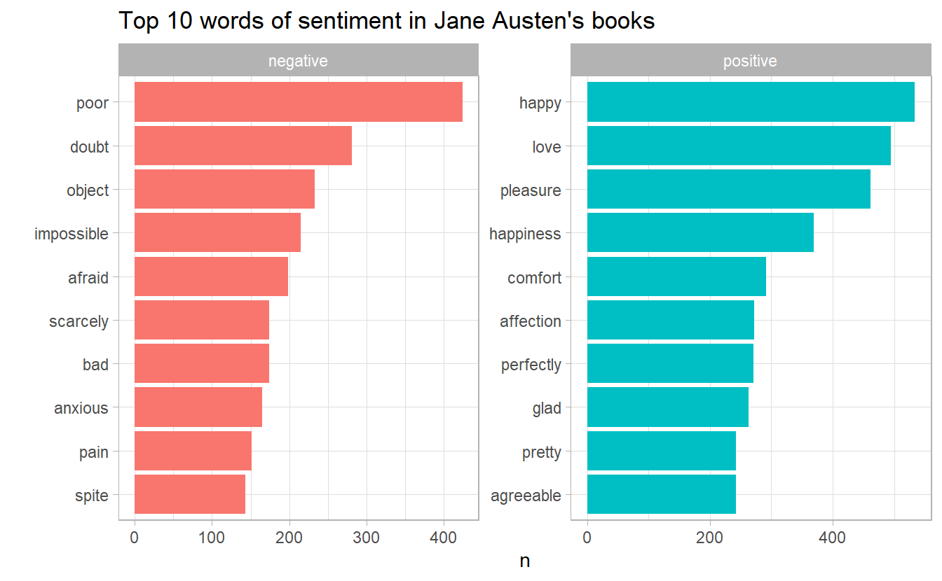
  ungroup()

Then we can make a bar plot

bing_word_counts %>%
  group_by(sentiment) %>% 
  top_n(10) %>%
  ungroup()  %>% 
  facet_bar(y = word, x = n, by = sentiment, nrow = 1) + 
  labs(title = "Top 10 words of sentiment in Jane Austen's books")