4.2 Counting and correlating pairs of words with widyr

Tokenizing by n-gram is a useful way to explore pairs of adjacent words. However, we may also be interested in words that tend to co-occur within particular documents or particular chapters, even if they don’t occur next to each other.

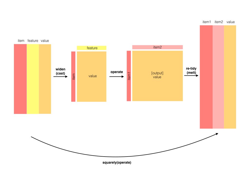
For this reason, it is sometimes necessary to “cast” a tidy dataset into a wide matrix (such as a co-occurrence matrix), performs an operation such as a correlation on it, then re-tidies the result. This is when widyr comes to the rescue, the workflow is shown in the book:

4.2.1 Counting and correlating among sections

We devide the book “Pride and Prejudice” into 10-line sections , as we did for Section 2.2 (80 lines). We may be interested in what words tend to appear within the same section.

austen_section_words <- austen_books() %>%
  filter(book == "Pride & Prejudice") %>%
  mutate(section = row_number() %/% 10) %>%
  filter(section > 0) %>%
  unnest_tokens(word, text) %>%
  filter(!word %in% stop_words$word)

austen_section_words
#> # A tibble: 37,240 x 3
#>   book              section word        
#>   <fct>               <dbl> <chr>       
#> 1 Pride & Prejudice       1 truth       
#> 2 Pride & Prejudice       1 universally 
#> 3 Pride & Prejudice       1 acknowledged
#> 4 Pride & Prejudice       1 single      
#> 5 Pride & Prejudice       1 possession  
#> 6 Pride & Prejudice       1 fortune     
#> # ... with 3.723e+04 more rows

widyr::pairwise_counts() counts the number of times each pair of items appear together within a group defined by “feature”. In this case, it counts the number of times each pair of words appear together within a section, note it still returns a tidy data frame, although the underlying computation took place in a matrix form :

library(widyr)

austen_section_words %>% 
  pairwise_count(word, section, sort = TRUE)
#> # A tibble: 796,008 x 3
#>   item1     item2         n
#>   <chr>     <chr>     <dbl>
#> 1 darcy     elizabeth   144
#> 2 elizabeth darcy       144
#> 3 miss      elizabeth   110
#> 4 elizabeth miss        110
#> 5 elizabeth jane        106
#> 6 jane      elizabeth   106
#> # ... with 7.96e+05 more rows

We can easily find the words that most often occur with Darcy. Since pairwise_count records both the counts of (word_A, word_B) and (word_B, word_B), it does not matter we filter at item1 or item2

austen_section_words %>% 
  pairwise_count(word, section, sort = TRUE) %>% 
  filter(item1 == "darcy")
#> # A tibble: 2,930 x 3
#>   item1 item2         n
#>   <chr> <chr>     <dbl>
#> 1 darcy elizabeth   144
#> 2 darcy miss         92
#> 3 darcy bingley      86
#> 4 darcy jane         46
#> 5 darcy bennet       45
#> 6 darcy sister       45
#> # ... with 2,924 more rows

4.2.2 Pairwise correlation

Pairs like “Elizabeth” and “Darcy” are the most common co-occurring words, but that’s not particularly meaningful since they’re also the most common individual words. We may instead want to examine correlation among words, which indicates how often they appear together relative to how often they appear separately.

In particular, we compute the \(\phi\) coefficient. Introduced by Karl Pearson, this measure is similar to the Pearson correlation coefficient in its interpretation. In fact, a Pearson correlation coefficient estimated for two binary variables will return the \(\phi\) coefficient. The phi coefficient is related to the chi-squared statistic for a 2 × 2 contingency table

\[ \phi = \sqrt{\frac{\chi^2}{n}} \]

where \(n\) denotes sample size. In the case of pairwise counts, \(\phi\) is calculated by

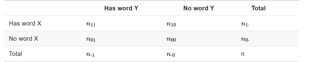
\[ \phi = \frac{n_{11}n_{00} - n_{10}n_{01}}{\sqrt{n_{1·}n_{0·}n_{·1}n_{·0}}} \]

We see, from the above quation, that \(\phi\) is “standarized” by individual counts, so various word pair with different individual frequency can be compared to each other:

The computation of \(\phi\) can be simply done by pairwise_cor (other choice of correlation coefficients specified by method). The procedure can be somewhat computationally expensive, so we filter out uncommon words

word_cors <- austen_section_words %>% 
  add_count(word) %>% 
  filter(n >= 20) %>% 
  select(-n) %>%
  pairwise_cor(word, section, sort = TRUE)

word_cors
#> # A tibble: 154,842 x 3
#>   item1    item2    correlation
#>   <chr>    <chr>          <dbl>
#> 1 bourgh   de             0.951
#> 2 de       bourgh         0.951
#> 3 pounds   thousand       0.701
#> 4 thousand pounds         0.701
#> 5 william  sir            0.664
#> 6 sir      william        0.664
#> # ... with 1.548e+05 more rows

Which word is most correlated with “lady”?

word_cors %>% 
  filter(item1 == "lady")
#> # A tibble: 393 x 3
#>   item1 item2     correlation
#>   <chr> <chr>           <dbl>
#> 1 lady  catherine       0.663
#> 2 lady  de              0.283
#> 3 lady  bourgh          0.254
#> 4 lady  ladyship        0.227
#> 5 lady  lucas           0.198
#> 6 lady  collins         0.176
#> # ... with 387 more rows

This lets us pick particular interesting words and find the other words most associated with them

word_cors %>%
  filter(item1 %in% c("elizabeth", "pounds", "married", "pride")) %>%
  group_by(item1) %>%
  top_n(6) %>%
  ungroup() %>%
  facet_bar(y = item2, x = correlation, by = item1)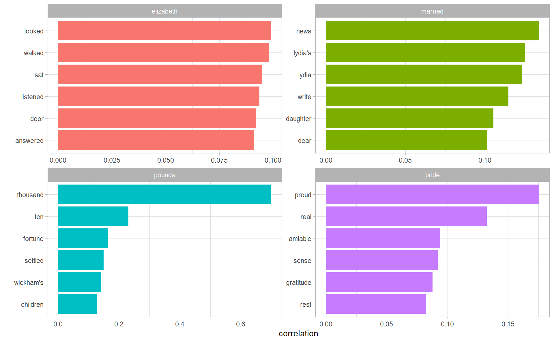

How about a network visualization to see the overall correlation pattern?

word_cors %>%
  filter(correlation > .15) %>%
  as_tbl_graph() %>%
  ggraph(layout = "fr") +
  geom_edge_link(aes(edge_alpha = correlation), show.legend = FALSE) +
  geom_node_point(color = "lightblue", size = 5) +
  geom_node_text(aes(label = name), repel = TRUE)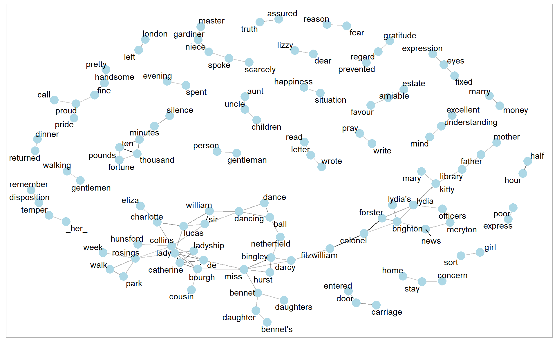

Note that unlike the bigram analysis, the relationships here are symmetrical, rather than directional (there are no arrows). We can also see that while pairings of names and titles that dominated bigram pairings are common, such as “colonel/fitzwilliam”, we can also see pairings of words that appear close to each other, such as “walk” and “park”, or “dance” and “ball”.