6.1 Latent Dirichlet Allocation

Latent Dirichlet allocation (LDA) is a particularly popular method for fitting a topic model. It treats each document as a mixture of topics, and each topic as a mixture of words. This allows documents to “overlap” each other in terms of content, rather than being separated into discrete groups, in a way that mirrors typical use of natural language.

The LDA model is guided by two principles:

Each document is a mixture of topics. In a 3 topic model we could assert that a document is 70% about topic A, 30 about topic B, and 0% about topic C.
Every topic is a mixture of words. A topic is considered a probabilistic distribution over multiple words.

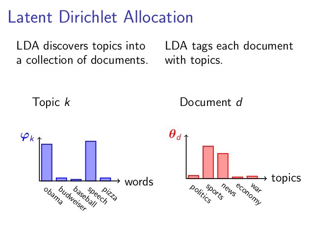
Figure 5.1: Source: http://nlpx.net/wp/wp-content/uploads/2016/01/LDA_image2.jpg

In particular, LDA is a imagined generative process, illustrated in the plate notation below:

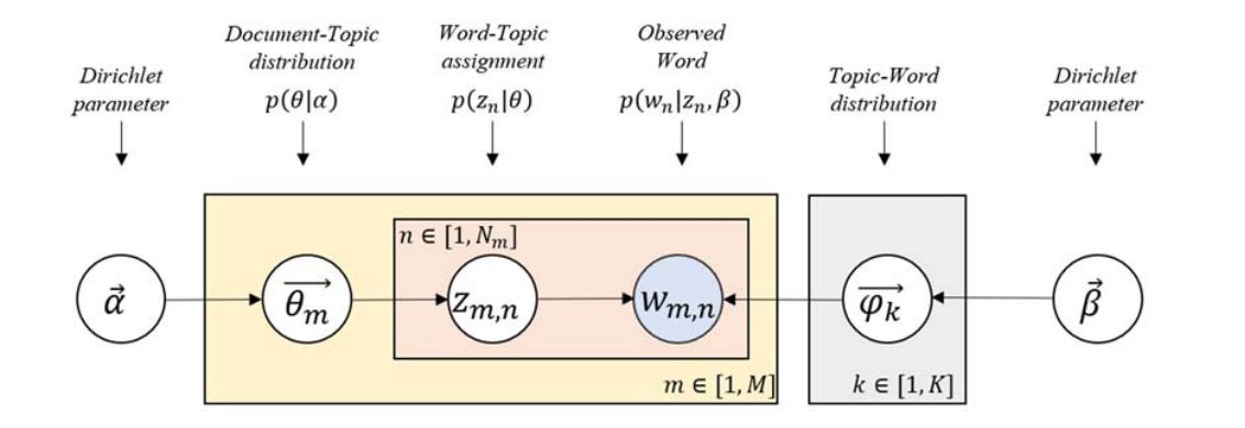
Figure 6.1: Source: Lee et al. (2018)

\(M\) denotes the number of documents
\(N\) is the number of words in a given document (document \(i\) has \(N_i\) words)
\(\vec{\theta_m}\) is the expected topic proportion of document \(m\), which is generated by a Dirichlet distribution parameterized by \(\vec{\alpha}\) (e.g., in a two topic model \(\theta_m = [0.3, 0.7]\) means document \(m\) is expected to have 30% topic 1 and 70% topic 2)
\(\vec{\phi_k}\) is the word distribution of topic \(k\), which is generated by a Dirichlet distribution parameterized by \(\vec{\beta}\)
\(z_{m, n}\) is the topic for the \(n\)th word in document \(m\), one word are assigned to one topic.
\(w_{m, n}\) is the word in the \(n\)th position word of document \(m\)

The only observed variable in this graphical probabilistic model is \(w_{m, n}\), so it is “latent”.

To actually infer the topics in a corpus, we imagine the generative process as follows. LDA assumes the following generative process for a corpus \(D\) consisting of \(M\) M documents each of length \(N_i\):

Generate \(\vec{\theta_i} \sim \text{Dir}(\vec{\alpha})\), where \(i \in \{1, 2, ..., M\}\). \(\text{Dir}(\vec{\alpha})\) is a Dirichlet distribution with symmetric parameter \(\vec{\alpha}\) where \(\vec{\alpha}\) is often sparse.
Generate \(\vec{\phi_k} \sim \text{Dir}(\vec{\beta})\), where \(k \in \{1, 2, ..., K\}\) and \(\vec{\beta}\) is typically sparse
For the \(n\)th position in document \(m\), where \(n \in \{1, 2, ..., N_m\}\) and \(m \in \{1, 2, ..., M\}\)
1. Choose a topic \(z_{m, n}\) for that position which is generated from \(z_{m, n} \sim \text{Multinomial}(\vec{\theta_i})\)
2. Fill in that position with word \(w_{m, n}\) which is generated from the word distribution of the topic picked in the previous step \(w_{i,j} \sim \text{Multinomial}(\phi_{z_{m, n}})\)

6.1.1 Example: Associated Press

We come to the AssociatedPress document term matrix (the required data strcture for the modeling function) and fit a two topic LDA model with stm::stm (stm stands for structural equation modeling). The stm takes as its input a document-term matrix, either as a sparse matrix (using cast_sparse) or a dfm from quanteda (using cast_dfm). Here we specify a two topic model by setting \(K = 2\) for demonstration purposes, in 6.3 we will see how to choose \(K\) with metrics such as semantic coherence.

library(stm)
data("AssociatedPress", package = "topicmodels")

ap_dfm <- tidy(AssociatedPress) %>% 
  cast_dfm(document = document, term = term, value = count)

ap_lda <- stm(ap_dfm, 
              K = 2, 
              verbose = FALSE, 
              init.type = "LDA")
summary(ap_lda)
#> A topic model with 2 topics, 2246 documents and a 10473 word dictionary.
#> Topic 1 Top Words:
#>       Highest Prob: i, people, two, police, years, officials, government 
#>       FREX: police, killed, miles, attorney, death, army, died 
#>       Lift: accident, accusations, ackerman, adams, affidavit, algotson, alice 
#>       Score: police, killed, trial, prison, died, army, hospital 
#> Topic 2 Top Words:
#>       Highest Prob: percent, new, million, year, president, bush, billion 
#>       FREX: percent, bush, billion, market, trade, prices, economic 
#>       Lift: corporate, growth, lawmakers, percentage, republicans, abboud, abm 
#>       Score: percent, billion, dollar, prices, yen, stock, market

stm objects have a summary() method for displaying words with highest probability in each topic. But we want to go back to data frames to take advantage of dplyr and ggplot2. For tidying model objects, tidy(model_object, matrix = "beta") (the default) access the topic-word probability vector (we denotes with \(\vec{\phi_k}\))

tidy(ap_lda)
#> # A tibble: 20,946 x 3
#>   topic term            beta
#>   <int> <chr>          <dbl>
#> 1     1 aaron     0.0000324 
#> 2     2 aaron     0.0000117 
#> 3     1 abandon   0.00000654
#> 4     2 abandon   0.0000676 
#> 5     1 abandoned 0.000140  
#> 6     2 abandoned 0.0000341 
#> # ... with 20,940 more rows

Which words have a relateve higher probabiltity to appear in each topic?

tidy(ap_lda) %>% 
  group_by(topic) %>%
  top_n(10) %>% 
  ungroup() %>% 
  mutate(topic = str_c("topic", topic)) %>%
  facet_bar(y = term, x = beta, by = topic) +
  labs(title = "Words with highest probability in each topic")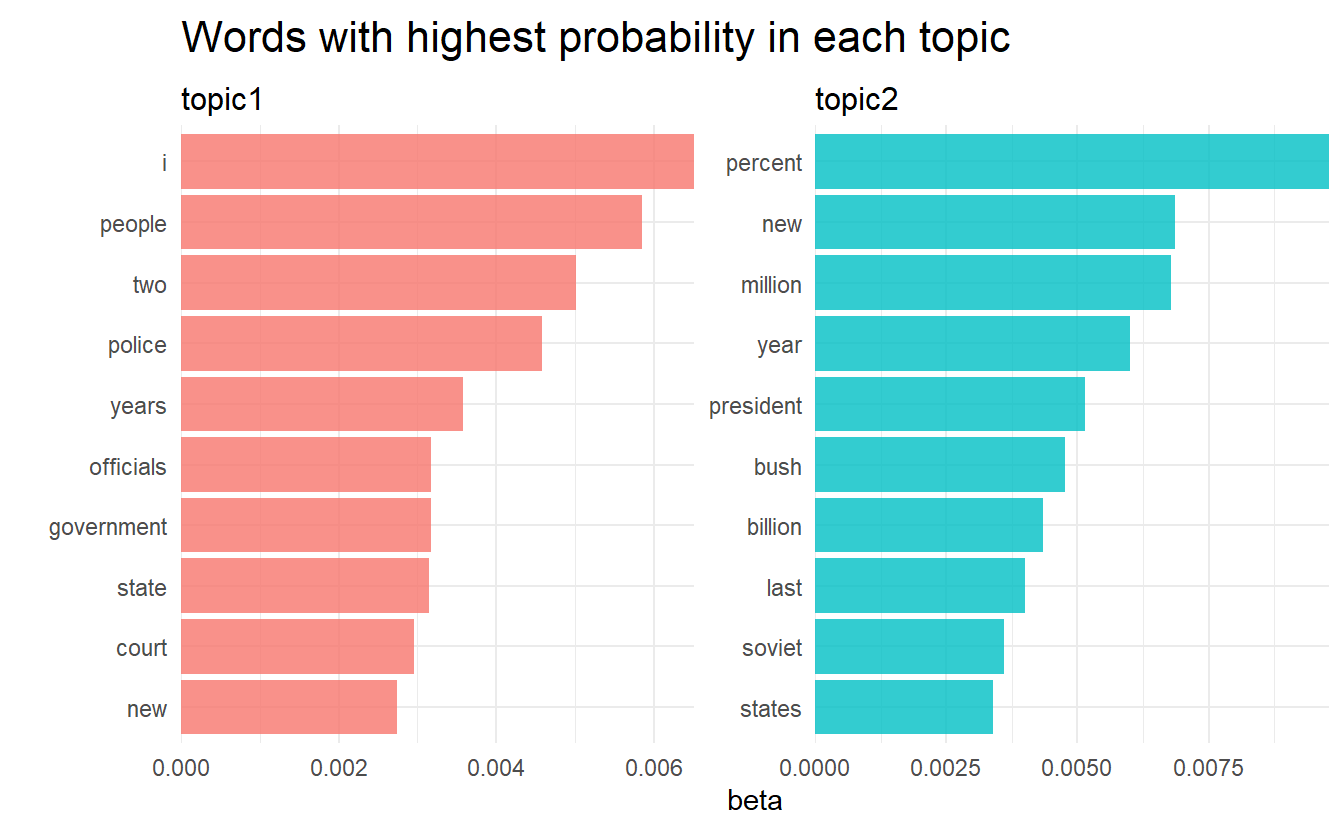

As an alternative, we could consider the terms that had the greatest difference in \(\vec{\phi_k}\) between topic 1 and topic 2. This can be estimated based on the log ratio of the two: \(\log_2(\frac{\phi_{1n}}{\phi_{2n}})\), \(\phi_{1n} / \phi_{2n}\) being the probability ratio of the sam e word \(n\) in two topics (a log ratio is useful because it makes the difference symmetrical)

phi_ratio <- tidy(ap_lda) %>%
  mutate(topic = str_c("topic", topic)) %>% 
  pivot_wider(names_from = topic, values_from = beta) %>% 
  filter(topic1 > .001 | topic2 > .001) %>%
  mutate(log_ratio = log2(topic2 / topic1))

This can answer a question like: which word is most representative of a topic?

phi_ratio %>% 
  top_n(20, abs(log_ratio)) %>% 
  ggplot(aes(y = fct_reorder(term, log_ratio),
             x = log_ratio)) + 
  geom_col() + 
  labs(y = "",
       x = "log ratio of phi between topic 2 and topic 1 (base 2)")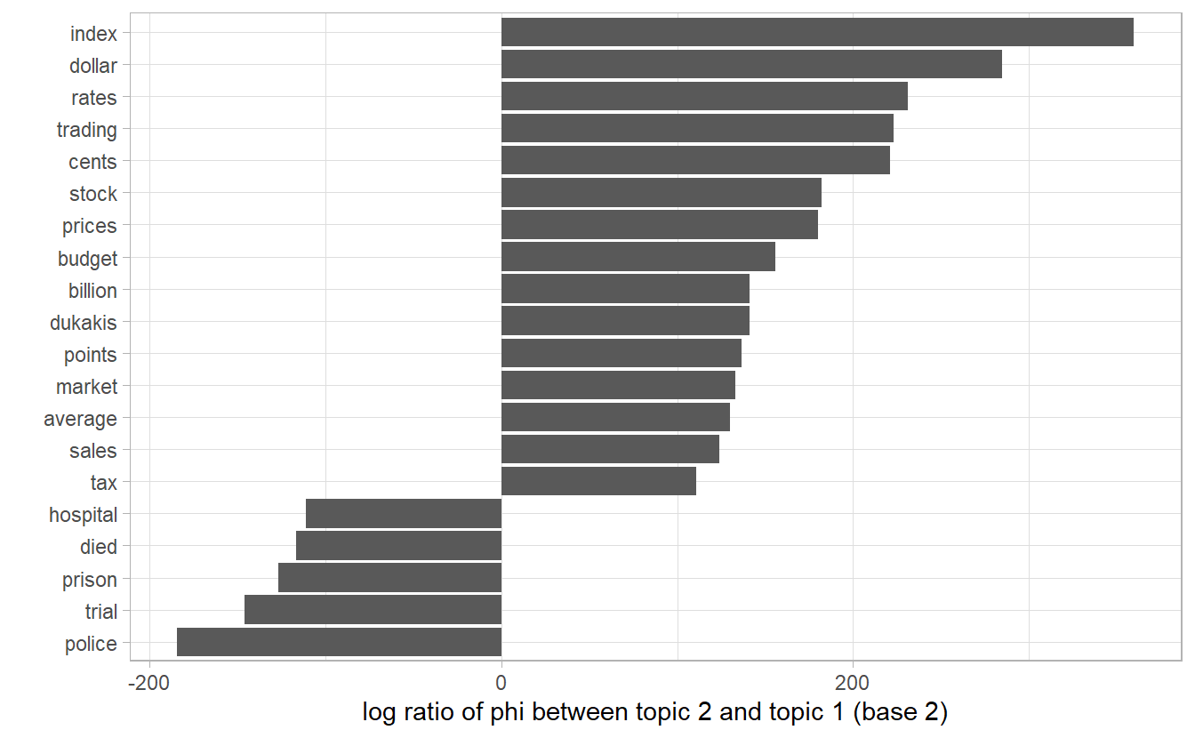

To extrac the word proportion vector \(\vec{\theta_m}\) for document \(m\), use matrix = "gamma" in tidy()

tidy(ap_lda, matrix = "gamma")
#> # A tibble: 4,492 x 3
#>   document topic gamma
#>      <int> <int> <dbl>
#> 1        1     1 0.990
#> 2        2     1 0.610
#> 3        3     1 0.983
#> 4        4     1 0.698
#> 5        5     1 0.891
#> 6        6     1 0.519
#> # ... with 4,486 more rows

With this data frame, we want to knwo which document is most charateristic of each topic?

library(reshape2)
library(wordcloud)

tidy(ap_lda, matrix = "gamma") %>% 
  group_by(topic) %>%
  top_n(15) %>% 
  mutate(document = as.character(document)) %>% 
  acast(document ~ topic, value.var = "gamma", fill = 0) %>% 
  comparison.cloud(colors = c("gray20", "gray80"), scale = c(2, 8))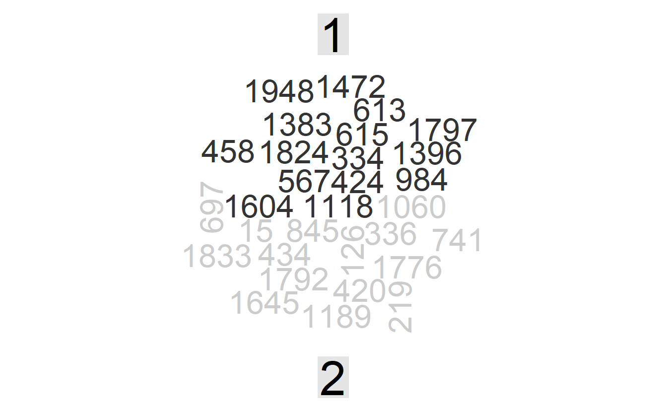

This plot would definitely be more insightful if we have document titles rather than an ID.

To sum up, the topic modeling workflow involves:
- use tidy tools like dplyr, tidyr, and ggplot2 for initial data exploration and preparation.
- cast to a non-tidy structure to perform some machine learning algorithm. - tidy the modeling results to to use tidy tools again (exploring, visualization, etc.)