14.4 Mediation

In mediation models (Baron and Kenny 1986), we want to examine if a direct effect from one variable to another is mediated by an intervening or mediator variable. If a total mediation exists, we assume that a variable \(X\) has an effect on a variable \(Y\) only because \(X\) influences a mediating variable \(Z\), which itself affects \(Y\).
Mediation is used in many fields, especially when we are interested in the mechanisms behind some relationship between two variables. However, it is important to mention that mediation models should always be based on a theoretically and logically sound rationale why the some variable \(Z\) is mediating the relationship between \(X\) and \(Y\).
Using meta-analytic SEM, we can synthesize evidence from original studies to determine if a proposed mediation is indeed backed by all available evidence. In the following, we will show you an example of how this can be done in R using the metaSEM package.
14.4.1 Model Specification
For this example, let us assume we want to disentangle why there is a relationship between (low) psychological resilience (see Fletcher and Sarkar (2013) for a definition of this concept) and elevated levels of depressive symptoms. Based on the literature, we assume that there are two mediating variables: emotion regulation capabilities and dysfunctional coping styles. Both mediating variables are influenced by resilience, while low emotion regulation capabilities also influence dysfunctional coping. Both emotion regulation and coping style then influence the level of depressive symptoms a person experiences. One may represent the proposed model graphically like this (again using idiosyncratic notation to facilitate the model specification later on):

For this example, we ill use the fictitious dat.med dataset, which was adapted from the Hunter83 dataset in metaSEM. The data can be downloaded here. The dataset is again a list containing (1) 14 correlation matrices for resilience, emotion regulation, dysfunctional coping and depressive symptoms extracted from 14 independent studies and (2) the \(N\) of each study (see previous chapter for more details on the dataset structure required). Let us have a look at the matrix for the fictitious Devegvar et al. (1992) study:
dat.med$data$`Devegvar et al. (1992)`## Resilience EmotReg Coping Depression
## Resilience NA NA NA NA
## EmotReg NA 1.00 0.72 0.05
## Coping NA 0.72 1.00 0.32
## Depression NA 0.05 0.32 1.00We see that this study has some missings, because the variable Resilience was not assessed. To see the overall missing data pattern, we can use the pattern.na() function.
pattern.na(dat.med$data)## Resilience EmotReg Coping Depression
## Resilience 1 3 3 2
## EmotReg 3 2 4 3
## Coping 3 4 2 3
## Depression 2 3 3 1We see that the correlation \(r_{EmotReg,Coping}\) has the most missings in our data, with four studies not providing data for it. Given that we have \(k=14\) studies overall, this amount of missing data may be acceptable. However, we have to check if the matrices are positive definite, because this is a requirement for the later processing steps. We can do this with the is.pd() function.
is.pd(dat.med$data)## Guttman et al. (2003) McCaffrey et al. (2002) Loescher et al. (1997)
## TRUE TRUE TRUE
## O'Malley et al. (1999) Hay et al. (1999) Twiraga et al. (2014)
## TRUE TRUE TRUE
## Wanzer et al. (1994) Arthur et al. (1991) Frondel et al. (1999)
## TRUE TRUE TRUE
## Mill et al. (2001) Ilan et al. (2002) Severence et al. (1996)
## TRUE TRUE TRUE
## Devegvar et al. (1992) Matloff et al. (2008)
## TRUE TRUEWe get TRUE for all studies, so everything is fine and we can continue.
14.4.2 Stage 1
Now let us proceed to pooling the correlation matrices in the first step. For a more detailed description of this step, please refer to the previous subchapter. This time, we use a fixed-effects model.
med1 <- tssem1(dat.med$data,
               dat.med$n,
               method = "FEM")

summary(med1)
##
## Call:
## tssem1FEM(Cov = Cov, n = n, cor.analysis = cor.analysis, model.name = model.name,
## cluster = cluster, suppressWarnings = suppressWarnings, silent = silent,
## run = run)
##
## Coefficients:
## Estimate Std.Error z value Pr(>|z|)
## S[1,2] 0.510487 0.012702 40.188 < 0.00000000000000022 ***
## S[1,3] 0.427086 0.014082 30.329 < 0.00000000000000022 ***
## S[1,4] 0.207713 0.015931 13.038 < 0.00000000000000022 ***
## S[2,3] 0.522965 0.013111 39.888 < 0.00000000000000022 ***
## S[2,4] 0.284562 0.015769 18.046 < 0.00000000000000022 ***
## S[3,4] 0.243256 0.016266 14.954 < 0.00000000000000022 ***
## ---
## Signif. codes: 0 '***' 0.001 '**' 0.01 '*' 0.05 '.' 0.1 ' ' 1
##
## Goodness-of-fit indices:
## Value
## Sample size 3975.0000
## Chi-square of target model 264.3980
## DF of target model 60.0000
## p value of target model 0.0000
## Chi-square of independence model 2777.2830
## DF of independence model 66.0000
## RMSEA 0.1096
## RMSEA lower 95% CI 0.0964
## RMSEA upper 95% CI 0.1234
## SRMR 0.0918
## TLI 0.9171
## CFI 0.9246
## AIC 144.3980
## BIC -232.8688
## OpenMx status1: 0 ("0" or "1": The optimization is considered fine.
## Other values may indicate problems.)The optimization status is 0, so the estimates are trustworthy. If you do not get a status of 0 or 1, plug the model into the rerun() function to try fitting it again.
14.4.3 Stage 2
Now that we have the pooled correlation matrix available in med1, we can proceed by specifying our proposed mediation model. Again, we specify the \(\mathbf{A}\) and \(\mathbf{S}\) matrices. The \(\mathbf{F}\) is not specified, because all of the variables in are model are observed (i.e., there are no latent variables). We will omit the details behind the matrix specification here; for more details please refer to the first subchapter for the general structure of the matrices, and the last subchapter on how the matrices are specified in R.
\[~\]
\(\mathbf{A}\) Matrix
We use starting values of \(0.2\).
# Build matrix
A <- matrix(c(0            , 0            , 0            , 0,
              "0.2*Res_EmR", 0            , 0            , 0,
              "0.2*Res_Cop", "0.2*EmR_Cop", 0            , 0,
              0            , "0.2*EmR_Dep", "0.2*Cop_Dep", 0),
              ncol = 4, nrow=4, byrow=TRUE)

# Set column and row labels
dimnames(A)[[1]] <- dimnames(A)[[2]] <- c("Resilience", "EmotReg", "Coping", "Depression")

A
## Resilience EmotReg Coping Depression
## Resilience "0" "0" "0" "0"
## EmotReg "0.2*Res_EmR" "0" "0" "0"
## Coping "0.2*Res_Cop" "0.2*EmR_Cop" "0" "0"
## Depression "0" "0.2*EmR_Dep" "0.2*Cop_Dep" "0"A <- as.mxMatrix(A)\[~\]
\(\mathbf{S}\) Matrix
We use starting values of \(0.1\).
# Build matrix
S <- Diag(c(1, "0.1*ErrVarE", "0.1*ErrVarC", "0.1*ErrVarD"))

# Set column and row labels
dimnames(S)[[1]] <- dimnames(S)[[2]] <- c("Resilience", "EmotReg", "Coping", "Depression")

S
## Resilience EmotReg Coping Depression
## Resilience "1" "0" "0" "0"
## EmotReg "0" "0.1*ErrVarE" "0" "0"
## Coping "0" "0" "0.1*ErrVarC" "0"
## Depression "0" "0" "0" "0.1*ErrVarD"S <- as.mxMatrix(S)\[~\]
Model Fitting
We can now proceed to fitting the model. In a mediation model, we also want to estimate the indirect effect from resilience to depression, taking all mediation paths into account. To do this, we can simply add all the mediation paths together. In our model, this would look like this:
\[\beta_{indirect_{Res-Dep}} = (\beta_{Res-Cop} \times \beta_{Cop-Dep}) + (\beta_{Res-EmR} \times \beta_{EmR-Cop} \times \beta_{Cop-Dep}) + (\beta_{Res-EmR} \times \beta_{Emr-Dep}) \]
We can define this function in our model so that it provides us with 95% confidence intervals around the indirect effect if we use likelihood-based intervals. We can define this function as a list containing an mxAlgebra object in R. Here is the code, using the labels we defined in the \(\mathbf{A}\) matrix above:
list(indirectEffect = mxAlgebra(Res_Cop*Cop_Dep + Res_EmR*EmR_Cop*Cop_Dep + Res_EmR*EmR_Dep,
                          name="indirectEffect"))
We can use this code as the argument for the mx.algebra parameter in our call to tssem2(). Because this is a mediation model, we also have to specify diag.constraints = TRUE. Here is the code:
med2 <- tssem2(med1,
               Amatrix = A,
               Smatrix = S,
               intervals.type = "LB",
               diag.constraints = TRUE,
               mx.algebras = list(indirectEffect = mxAlgebra(Res_Cop*Cop_Dep +
                                                    Res_EmR*EmR_Cop*Cop_Dep +
                                                    Res_EmR*EmR_Dep,
                                                   name="indirectEffect")))

# Rerun
med2 <- rerun(med2)

summary(med2)
Call:
wls(Cov = coef.tssem1FEM(tssem1.obj), aCov = vcov.tssem1FEM(tssem1.obj),
n = sum(tssem1.obj$n), Amatrix = Amatrix, Smatrix = Smatrix,
Fmatrix = Fmatrix, diag.constraints = diag.constraints, cor.analysis = tssem1.obj$cor.analysis,
intervals.type = intervals.type, mx.algebras = mx.algebras,
model.name = model.name, suppressWarnings = suppressWarnings,
silent = silent, run = run)
95% confidence intervals: Likelihood-based statistic
Coefficients:
Estimate Std.Error lbound ubound z value Pr(>|z|)
EmR_Cop 0.411161 NA 0.377782 0.444676 NA NA
Res_Cop 0.217913 NA 0.183661 0.252118 NA NA
Cop_Dep 0.131068 NA 0.091942 0.170226 NA NA
EmR_Dep 0.218838 NA 0.180424 0.257309 NA NA
Res_EmR 0.513365 NA 0.488406 0.538309 NA NA
ErrVarC 0.691468 NA 0.664472 0.717400 NA NA
ErrVarD 0.904928 NA 0.885399 0.922669 NA NA
ErrVarE 0.736457 NA 0.710223 0.761460 NA NA
mxAlgebras objects (and their 95% likelihood-based CIs):
lbound Estimate ubound
indirectEffect[1,1] 0.1498335 0.1685701 0.1878938
Goodness-of-fit indices:
Value
Sample size 3975.0000
Chi-square of target model 9.4087
DF of target model 1.0000
p value of target model 0.0022
Number of constraints imposed on "Smatrix" 3.0000
DF manually adjusted 0.0000
Chi-square of independence model 2697.6496
DF of independence model 6.0000
RMSEA 0.0460
RMSEA lower 95% CI 0.0226
RMSEA upper 95% CI 0.0748
SRMR 0.0161
TLI 0.9813
CFI 0.9969
AIC 7.4087
BIC 1.1209
OpenMx status1: 0 ("0" or "1": The optimization is considered fine.
Other values indicate problems.)Because we told the tssem2() function to use likelihood-based intervals, the Wald-type \(p\)-values are not displayed. We see that the proposed model fits the data closely, with \(\chi^{2}_{1,3975} = 9.4, p=0.002\)) and the \(RMSEA = 0.046\) being smaller than \(0.05\). Please note however, that we used the fixed-effect model in stage 1 to pool the correlations, which may not be appropriate if the between-study heterogeneity is substantial. The estimate of the indirect effect from resilience to depression assuming our moderation model is \(0.17\), which is significant (\(95\%CI: 0.15-0.19\)).
14.4.4 Plotting the Model
Again, we can plot our model using the semPaths() function in the semPlot package.
# Convert to semPlot
sem.plot <- meta2semPlot(med2)

# Create Labels (left to right, bottom to top)
labels <- c("Resilience","Emotion\nRegulation","Coping","Depres-\nsion")

# Plot
semPaths(sem.plot,
         whatLabels = "est",
         edge.color = "black",
         layout="tree2",
         rotation=2,
         nodeLabels = labels)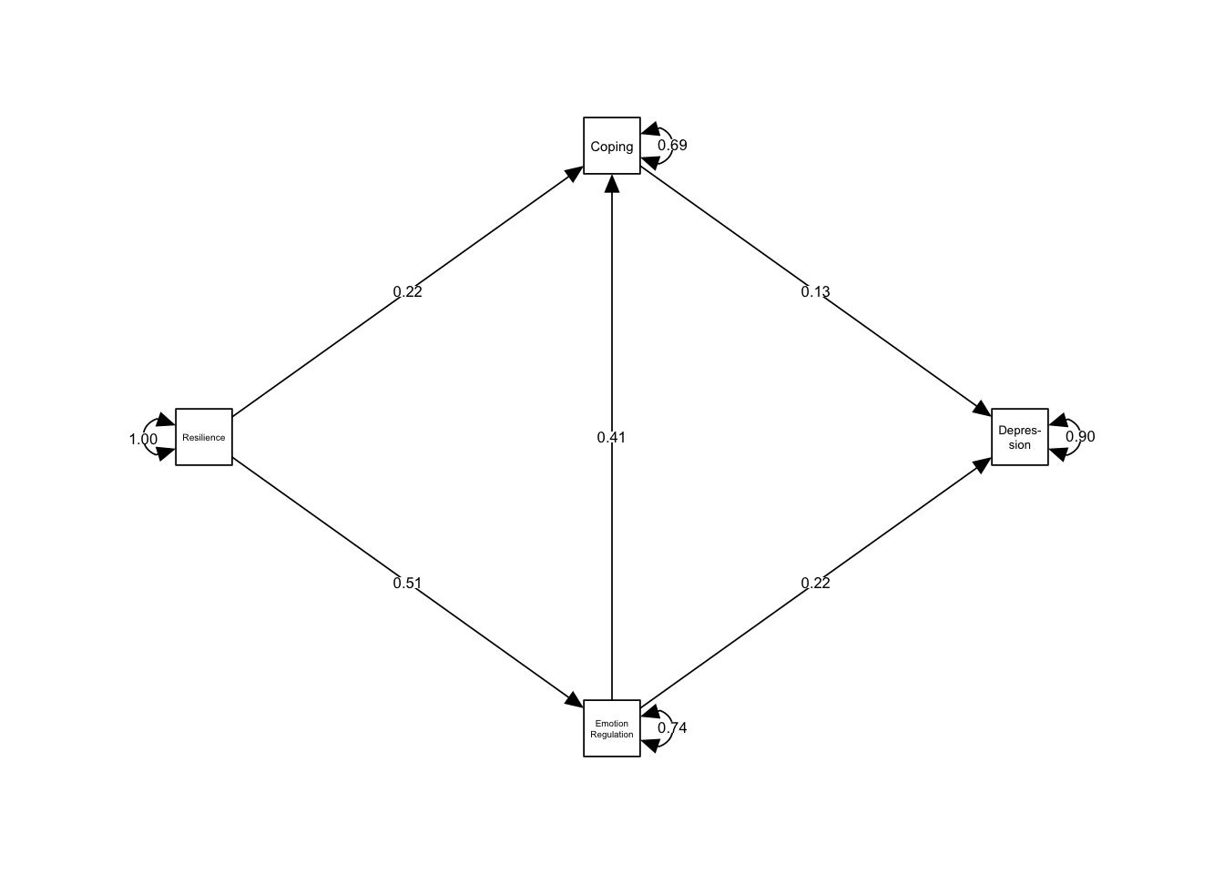
References
Baron, Reuben M, and David A Kenny. 1986. “The Moderator–Mediator Variable Distinction in Social Psychological Research: Conceptual, Strategic, and Statistical Considerations.” Journal of Personality and Social Psychology 51 (6). American Psychological Association: 1173.
Fletcher, David, and Mustafa Sarkar. 2013. “Psychological Resilience: A Review and Critique of Definitions, Concepts, and Theory.” European Psychologist 18 (1). Hogrefe Publishing: 12.
