11.2 Bayesian Network Meta-Analysis

In the following, we will describe how to perform a network meta-analysis based on a bayesian hierarchical framework. The R package we will use to do this is the gemtc package (Valkenhoef et al. 2012). But first, let us consider the idea behind bayesian in inference in general, and the bayesian hierarchical model for network meta-analysis in particular.
Bayesian Inference
Besides the frequentist framework, bayesian inference is another important strand of inference statistics. Although the frequentist approach is arguably used more often in most research fields, bayesian statistics is actually older, and despite being increasingly picked up by researchers in recent years (Marsman et al. 2017), has never really been “gone” (McGrayne 2011). The central idea of bayesian statistics revolves around Bayes’ Theorem, first formulated by Thomas Bayes (1701-1761). Bayesian statistics differs from frequentism because it also incorporates “subjective” prior knowledge into statistical inference. In particular, Bayes’ theorem allows us to estimate the probability of an event \(A\), given that we already know that another event \(B\) has occurred, or is the case. This is a conditional probability, which can be expressed like this in mathematical notation: \(P(A|B)\). Bayes’ theorem then looks like this:
\[P(A|B)=\frac{P(B|A)\times P(A)}{P(B)}\]
The two probabilities in the upper part of the fraction to the right have their own names. First, the \(P(B|A)\) part is (essentially) known as the likelihood; in our case, this is the probability of event \(B\) (which has already occurred), given that \(A\) is in fact the case, or occurs (Etz 2018). \(P(A)\) is the “prior” probability of \(A\) occurring. \(P(A|B)\), lastly, is the “posterior” probability. Given that \(P(B)\) is a fixed constant, the formula above is often shortened to this form:
\[P(A|B) \propto P(B|A)\times P(A)\]
Where the \(\propto\) sign means that now that we have discarded the denominator of the fraction, the probability on the left remains at least “proportional” to the part on the right with changing values (Shim et al. 2019). We may understand Bayes’ Theorem better if we think of the formula as a process, beginning on the right side of the equation. We simply combine the prior information we have on the probability of \(A\) occuring with the likelihood of \(B\) given that \(A\) actually occurs to produce our posterior, or adapted, probability of \(A\). The crucial point here is that we can produce a “better”, i.e. posterior, estimate of \(A\)’s probability when we take our previous knowledge of the context into account. This context knowledge is our prior knowledge on the probability of \(A\).
Bayes’ Theorem is often explained in the way we did above, with \(A\) and \(B\) standing for specific events. The example may become less abstract however, if we take into account that \(A\) and \(B\) can also represent distributions of a variable. Let us now assume that \(P(A)\) follows in fact a distribution. This distribution is characterized by a set of parameters which we denote by \(\theta\). For example, if our distribution follows a gaussian normal distribution, it can be described by its mean \(\mu\) and variance \(\sigma^2\). The \(\theta\) parameters is what we actually want to estimate. Now, let us also assume that, instead of \(B\), we have collected actual data through which we want to estimate \(\theta\). We store our observed data in a vector \(\bf{Y}\); of course, our observed data also follows a distribution, \(P(\bf{Y})\). The formula now looks like this:
\[P(\theta | {\bf{Y}} ) \propto P( {\bf{Y}} | \theta )\times P( \theta )\]
In this equation, we now have \(P(\theta)\), the prior distribution of \(\theta\), which we simply define a priori, either based on our previous knowledge, or even our intuition on what the \(\theta\) values may look like. Together with the likelihood distribution \(P({\bf{Y}}|\theta)\) of our data given the true parameters \(\theta\), we can estimate the posterior distribution \(P(\theta|{\bf{Y}})\), which represents what we think the \(\theta\) parameters look like if we take both the observed data and our prior knowledge into account. As can be seen in the formula, the posterior is still a distribution, not an estimated “true” value, meaning that even the results of bayesian inference are still probabilistic, and subjective in the sense that they represent our belief in the actual parameter values. Bayesian inference thus also means that we do not calculate confidence intervals around our estimates, but credibility intervals (CrI).
Here is a visualisation of the three distributions we described above, and how they might look like in a specific example:
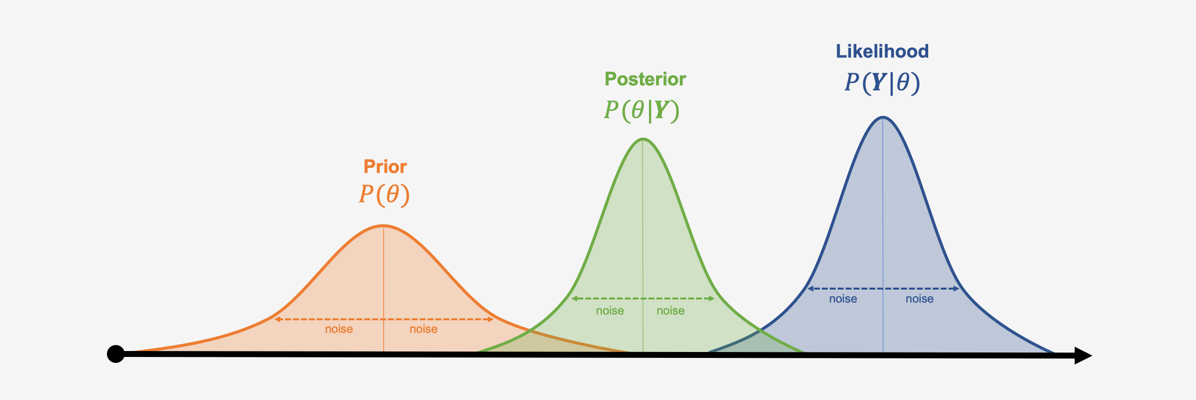
A big asset of bayesian approaches is that the distributions do not have to follow a bell curve distribution like the ones in our visualization; any other kind of (more complex) distribution can be modeled. A disadvantage of bayesian inference, however, is that generating the (joint) distribution parameters from our collected data can be very computationally intensive; special Markov Chain Monte Carlo simulation procedures, such as the Gibbs sampling algorithm have thus been developed to generate posterior distributions. Markov Chain Monte Carlo is also used in the gemtc package to build our bayesian network meta-analysis model (Valkenhoef et al. 2012).
11.2.1 The Network Meta-Analysis Model
We will now formulate the bayesian hierarchical model underlying the gemtc package. We will start by defining the model for a conventional pairwise meta-analysis. This definition of the meta-analysis model is equivalent with the one provided in Chapter 4.2, where we discuss the random-effects model. What we will describe is simply the bayesian way to conceptualize meta-analysis, and we use this other formulation so that you can more easily read up on the statistical background of bayesian network meta-analysis in other literature. On the other hand, the bayesian definition of pairwise meta-analysis is also highly important because it is directly applicable to network meta-analyses, without any further extension (Dias et al. 2013). The model used in the gemtc package is also called a bayesian hierarchical model (Efthimiou et al. 2016). There is nothing majorly complicated about the word hierarchical here; indeed we already described in Chapter 12 that even the most simple meta-analysis model presupposes a hierarchical, or “multilevel” structure.
11.2.1.1 The fixed-effect model
Suppose that we want to conduct a conventional pairwise meta-analysis. We have included \(K\) studies, and have collect an effect size \(Y_k\) for each of our studies \(k = 1,...,K\). We can then define the fixed-effect model like this:
\[Y_k \sim \mathcal{N}(\delta,s_k^2)\]
This formula expresses the likelihood (the \(P({\bf{Y}}|\theta)\) part from above) of our effect sizes, assuming that they follow a normal distribution. We assume that each effect size is a simply a draw from the distribution of the one true effect size \(\delta\), which has the variance \(s_k^2\). In the fixed-effect model, we assume that there is one true effect underlying all the effect sizes we observe, so \(\delta\) stays the same for different studies \(k\) and their corresponding observed effect sizes \(Y_k\). The interesting part in the bayesian model is that while the true effect \(\delta\) is unkown, we can still define a prior distribution defining how we think \(\delta\) may look like. For example, we could assume a prior following a normal distribution, \(\delta \sim \mathcal{N}(0,s^2)\), were we specify \(s^2\). The gemtc package by default uses so-called uninformative priors, which are prior distributions with a very large variance. This is done so that our prior “beliefs” do not have a big impact on the posterior results, and we only let the actual observed data “speak”.
11.2.1.2 The random-effects model
We can easily extend this formula for the random-effects model:
\[Y_k \sim \mathcal{N}(\delta_k,s_k^2)\]
Not much has changed here, except that now using the random-effects model, we do not assume that each study is an estimator of the one true effect size \(\delta\), but that there are study-specific true effects \(\delta_k\) estimated by each effect size \(Y_k\). Furthermore, these study-specific true effects are again part of an overarching distribution of true effect sizes, which is defined by its mean \(d\) and variance \(\tau^2\), our between-study heterogeneity.
\[\delta_k \sim \mathcal{N}(d,\tau^2)\] In the bayesian model, we also give a (uninformative) prior distribution to both \(d\) and \(\tau^2\).
11.2.1.3 Application to network meta-analysis
Now that we have covered how a bayesian meta-analysis model can be formulated for pairwise meta-analysis, we can start to apply this model to the network meta-analysis context. The random-effect model formula above can be directly used to achieve this - we only have to conceptualize our model parameters a little differently. Now that we also want to make clear that comparisons in network meta-analysis can consist of different treatments being compared, we can denote a single effect size we have obtained from one study \(k\) as \(Y_{kab}\), which signifies that for this effect size in study \(k\), treatment \(a\) was compared to treatment \(b\). If we apply this new notation to the entire formula, we get this:
\[Y_{kab} \sim \mathcal{N}(\delta_{kab},s_k^2)\] \[\delta_{kab} \sim \mathcal{N}(d_{ab},\tau^2)\] We see that the formulae still follow the same concept as before, but now we assume that our study-specific “true” effect for the comparison of \(a\) and \(b\) is assumed to be part of an overarching distribution of true effect sizes with mean \(d_{ab}\). This mean true effect size \(d_{ab}\) of the \(a-b\) comparison is in fact the result of subtracting \(d_{1a}-d_{1b}\), where \(d_{1a}\) is the effect of treatment \(a\) compared to some predefined reference treatment \(1\), and \(d_{1b}\) is the effect of treatment \(b\) compared to the same reference treatment. In the bayesian model, these effects compared to the reference group are also given a prior distribution.
As we have already mentioned in the previous chapter on frequentist network meta-analysis, combining multiarm studies into our network model is problematic because these treatment arms are correlated. In the bayesian framework, this issue is solved by assuming that the effects of the \(i\) treatments contained in the \(i+1\) treatment arms of some multiarm study \(k\) stem from a multivariate normal distribution:
\[\begin{align} \left( \begin{array}{c} \delta_{kab1} \\ \delta_{kab1} \\ \delta_{kab3} \\ \vdots \\ \delta_{kabi} \\ \end{array} \right) = \mathcal{N} \left( \left( \begin{array}{c} d_{ab1} \\ d_{ab1} \\ d_{ab3} \\ \vdots \\ d_{abi} \\ \end{array} \right) , \left( \begin{array}{ccccc} \tau^2 & \tau^{2}/2 & \tau^{2}/2 & \cdots & \tau^{2}/2\\ \tau^{2}/2 & \tau^2 & \tau^{2}/2 & \cdots & \tau^{2}/2\\ \tau^{2}/2 & \tau^{2}/2 & \tau^2 & \cdots & \tau^{2}/2\\ \vdots & \vdots & \vdots & \ddots & \vdots\\ \tau^{2}/2 & \tau^{2}/2 & \tau^{2}/2 & \cdots & \tau^2\\ \end{array} \right) \right) \end{align}\]
11.2.2 Performing a Network Meta-Analysis using the gemtc package
Now, let us start using the gemtc package to perform our first bayesian network meta-analysis. As always, we have to first install the package, and then load it from our library.
install.packages("gemtc")
library(gemtc)
The gemtc also requires the rjags package, which is used for the Gibbs sampling procedure we described above, to function properly. However, before we install and load this package, we also have to install a software called JAGS (short for “Just Another Gibbs Sampler”) on our computer. The software is available for both Windows and Mac/Unix, and you can download it for free here.
After this is done, we can also install and load the rjags package.
install.packages("rjags")
library(rjags)
11.2.2.1 Data preprocessing
Now, let us restructure our data so that functions of the gemtc package can process it. Like in the chapter on frequentist network meta-analysis, we will use the data by Senn2013 comparing different medications for diabetic patients for our analysis.
However, we had to tweak the structure of our data little to conform with gemtcs requirements. The original dataset contains the Mean Difference (TE) between two treatments, with each row representing one comparison. However, for the gemtc package, we need to reshape our data so that each row represents a single treatment arm. Furthermore, we have to specify which treatment arm was the reference group for the effect size calculated for a comparison by giving it the label “NA”. Here is how our reshaped dataset looks like, which we again called data:
The gemtc package also requires that the columns of our dataframe are labeled correctly. If we have precalculated effect sizes for continuous outcomes (such as the Mean Difference or Standardized Mean Difference), our dataset has to contain these columns:
- study. This columns contains the (unique) label for each study included in our network, equivalent to the “studlab” column used in
netmeta. - treatment. This column contains the label for the treatment.
- diff. This column contains the effect size (e.g., the mean difference calculated for a comparison). Importantly, the diff column contains “NA”, a missing, in the row of the reference treatment of a specific study. The row of the treatment to which the reference treatment was compared to then holds the actual effect size calculated for this comparison. Also keep in mind that the reference category is defined study-wise, not comparison-wise. This means that in multiarm studies, we still have only one reference treatment to which the other treatments are compared.
- std.err. This column contains the standard error of the effect sizes, and follows the same pattern.
Please note that other data formats are also possible, for example for binary outcome or other raw effect size data. The way your dataset needs to be structured in such cases is described here and here.
11.2.2.2 Network graph
Now that we have our data ready, we feed it to the mtc.network() function to generate an element of class mtc.network, which we can use for later modeling steps. Because we are using precalculated effect size data, we have to specify our dataset with the data.re parameter. For raw effect size data (e.g. Mean, SD, N), we would have used the data.ab argument. We save the result as network.
network <- mtc.network(data.re = data)Plugging the resulting network object into the summary() function already provides us with some interesting information about the structure of our network.
summary(network)## $Description
## [1] "MTC dataset: Network"
##
## $`Studies per treatment`
## Acarbose Benfluorex Metformin Miglitol Pioglitazone
## 3 2 8 3 3
## Placebo Rosiglitazone Sitagliptin Sulfonylurea Vildagliptin
## 19 10 1 3 1
##
## $`Number of n-arm studies`
## 2-arm 3-arm
## 25 1
##
## $`Studies per treatment comparison`
## t1 t2 nr
## 1 Acarbose Metformin 1
## 2 Acarbose Placebo 2
## 3 Acarbose Sulfonylurea 1
## 4 Benfluorex Placebo 2
## 5 Metformin Pioglitazone 1
## 6 Metformin Placebo 4
## 7 Metformin Rosiglitazone 2
## 8 Metformin Sulfonylurea 1
## 9 Miglitol Placebo 3
## 10 Pioglitazone Placebo 1
## 11 Pioglitazone Rosiglitazone 1
## 12 Placebo Rosiglitazone 6
## 13 Placebo Sitagliptin 1
## 14 Placebo Vildagliptin 1
## 15 Rosiglitazone Sulfonylurea 1We can also use the plot() function to generate our network plot. Like the network generated by the netmeta package, the network’s edge thickness corresponds with the number of studies we have for that comparison.
plot(network)
As an alternative, we can also check if we can create a better visualisation of our network using the Fruchterman-Reingold algorithm. This algorithm comes with some inherent randomness, meaning that we can rerun the code below several times to get different results (make sure to have the igraph package installed and loaded for this to work).
plot(network, layout=layout.fruchterman.reingold)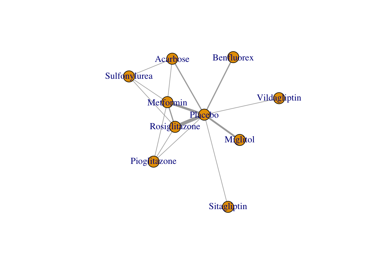
11.2.2.3 Model compilation
Using our mtc.network() object network, we can now start to specify and compile our model. The great thing about the gemtc package is that is automates most parts of the bayesian inference process, for example by choosing adequate prior distributions for all parameters in our model.
Thus, there are only a few parameters we have to specify when compiling our model using the mtc.model() function. First, we have to specify the mtc.network() object we have created before. Furthermore, we have to specify if we want to use a random- or fixed effects model using the linearModel argument. Given that our previous frequentist analysis indicated substantial heterogeneity and inconsistency, we will set linearModel = "random". Lastly, we also have to specify the number of Markov chains we want to use. A value between 3 and 4 is sensible here, and we will chosse n.chain = 4. We call our compiled model model.
model <- mtc.model(network,
                   linearModel = "random",
                   n.chain = 4)
11.2.2.4 Markov Chain Monte Carlo simulation
Now we come to the crucial part of our analysis: the Markov Chain Monte Carlo simulation, which will allows to estimate the posterior distributions of our parameters, and thus generate the results of our network meta-analysis. There are two important desiderata we want to achieve for our model using this procedure:
- We want that the first few runs of the Markov Chain Monte Carlo simulations, which will likely produce inadequate results, do not have a large impact on the whole simulation results.
- We want the Markov Chain Monte Carlo process to run long enough for us to reach accurate estimates of our parameters (i.e., to reach convergence).
To address these points, we split the number of times the Markov Chain Monte Carlo algorithm iterates over our data to infer the model results into two phases: first, we define the number of burn-in iterations (n.adapt), the results of which are then discarded. For the following phase, we can specify the number of actual simulation iterations (n.iter), which we use for the model inference. Given that we often simulate many, many iterations, we can also specify the thin argument, which allows us to only extract the values of every \(i\)th iteration, which makes our simulation less computationally intensive.
The simulation can be performed using the mtc.run() function. In our example, we will perform two seperate simulations with different settings to compare which one works the best. We have to provide the function with our compiled model object, and we have to specify the parameters we described above. We conduct a first simulation with less iterations, and then a second simulation in which we increase the number of iterations. We save these objects as mcmc1 and mcmc2. Depending on the size of your network, the simulation may take some time to finish.
mcmc1 <- mtc.run(model, n.adapt = 50, n.iter = 1000, thin = 10)
mcmc2 <- mtc.run(model, n.adapt = 5000, n.iter = 100000, thin = 10)
11.2.2.5 Assessing the convergence
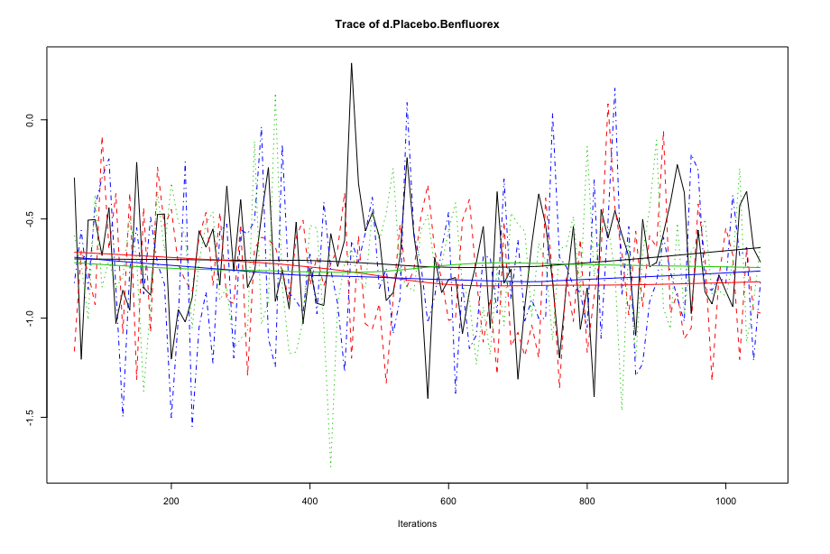
To see if our simulations have resulted in the convergence of the algorithm, and to check which settings are preferable, we can evaluate some of the outputs of our mcmc1 and mcmc2 objects. A good start is to use the plot() function. This provides us with a “time series”, commonly referred to as a trace plot, for each treatment comparison over all iterations. For now, we only focus on the comparison Placebo vs. Benfluorex.
Here is the trace plot for mcmc1.
And this is the trace plot for mcmc2.
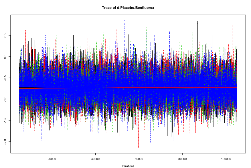
When comparing earlier iterations to later iterations in the first plots, we see that there is some discontinuity in the overall trend of the time series, and that the estimates of the four different chains (the four solid lines) differ in their course when moving from the first half to the second half of the plot. In the plot for our second simulation, on the other hand, we see much more rapid up-and-down variation, but no real long-term trend. This delivers a first indication that the settings of mcmc2 are more adequate.
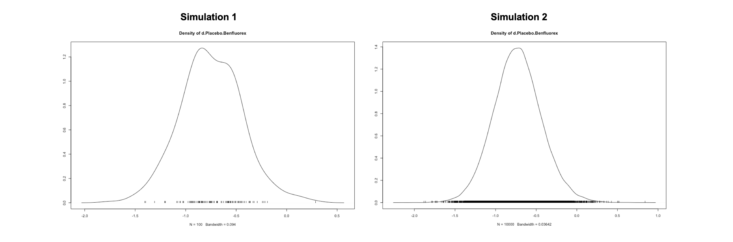
We can continue with our convergence evaluation by looking at the density plots of our posterior effect size estimate. We see that while the distribution resulting from mcmc1 still diverges considerably from a smooth normal distribution, the result of mcmc2 looks much more like this.
Another highly helpful method to assess convergence is the Gelman-Rubin-Brooks plot. This plot shows the so-called Potential Scale Reduction Factor (PSRF), which compares the variation within each chain in simulation to the variation between chains, and how it develops over time. In case of convergence, the PRSF should gradually shrink down to zero with increasing numbers of interations, and should at least be below 1.05 in the end. To produce this plot, we simply have to plug in the mtc.run() object into the gelman.plot() function. Here is there result for both simulations.
gelman.plot(mcmc1)
gelman.plot(mcmc2)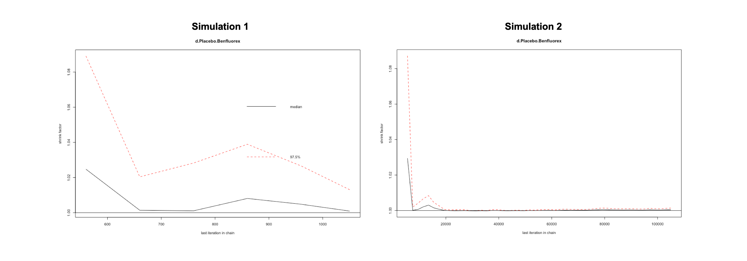
We can also directly access the overall PSRF of our model results using this code:
gelman.diag(mcmc1)$mpsrf## [1] 1.055129gelman.diag(mcmc2)$mpsrf## [1] 1.000689We see that the overall PRSF is only below the threshold for our second simulation mcmc2, indicating that we should use the results obtained by this simulation.
11.2.3 Assessing inconsistency: the nodesplit method
Like the netmeta package, the gemtc package also provides us with a way to evaluate the consistency of our network model, using the nodesplit method. The idea behind the procedure we apply here equals the one of the net splitting method we described before. To perform a nodesplit analysis, we use the mtc.nodesplit() function, using the same settings as used for mcmc2. We save the result as nodesplit.
Be aware that the nodesplit computation may take a long time, even up to hours, depending on the complexity of your network.
nodesplit <- mtc.nodesplit(network,
                          linearModel = "random",
                          n.adapt = 5000,
                          n.iter = 100000,
                          thin = 10)
The best way to interpret the results of our nodesplit model is to plug it into the summary function.
summary(nodesplit)## Node-splitting analysis of inconsistency
## ========================================
##
## comparison p.value CrI
## 1 d.Acarbose.Metformin 0.79900
## 2 -> direct -0.20 (-0.95, 0.55)
## 3 -> indirect -0.32 (-0.99, 0.36)
## 4 -> network -0.28 (-0.77, 0.22)
## 5 d.Acarbose.Placebo 0.92395
## 6 -> direct 0.86 (0.20, 1.5)
## 7 -> indirect 0.80 (-0.25, 1.8)
## 8 -> network 0.85 (0.36, 1.3)
## 9 d.Acarbose.Sulfonylurea 0.90455
## 10 -> direct 0.40 (-0.39, 1.2)
## 11 -> indirect 0.46 (-0.34, 1.3)
## 12 -> network 0.43 (-0.11, 0.97)
## 13 d.Metformin.Pioglitazone 0.53465
## 14 -> direct 0.16 (-0.58, 0.90)
## 15 -> indirect -0.13 (-0.78, 0.52)
## 16 -> network -0.00017 (-0.49, 0.47)
## 17 d.Metformin.Placebo 0.74040
## 18 -> direct 1.2 (0.71, 1.6)
## 19 -> indirect 1.1 (0.54, 1.6)
## 20 -> network 1.1 (0.80, 1.4)
## 21 d.Metformin.Rosiglitazone 0.86175
## 22 -> direct -0.069 (-0.67, 0.53)
## 23 -> indirect -0.13 (-0.58, 0.29)
## 24 -> network -0.11 (-0.46, 0.23)
## 25 d.Metformin.Sulfonylurea 0.20050
## 26 -> direct 0.37 (-0.35, 1.1)
## 27 -> indirect 0.97 (0.33, 1.6)
## 28 -> network 0.71 (0.22, 1.2)
## 29 d.Pioglitazone.Placebo 0.53095
## 30 -> direct 1.3 (0.55, 2.1)
## 31 -> indirect 1.0 (0.42, 1.6)
## 32 -> network 1.1 (0.66, 1.6)
## 33 d.Pioglitazone.Rosiglitazone 0.98445
## 34 -> direct -0.10 (-0.92, 0.71)
## 35 -> indirect -0.11 (-0.71, 0.50)
## 36 -> network -0.11 (-0.58, 0.37)
## 37 d.Placebo.Rosiglitazone 0.46620
## 38 -> direct -1.2 (-1.5, -0.87)
## 39 -> indirect -1.4 (-1.9, -0.85)
## 40 -> network -1.2 (-1.5, -0.97)
## 41 d.Rosiglitazone.Sulfonylurea 0.14985
## 42 -> direct 1.2 (0.48, 1.9)
## 43 -> indirect 0.51 (-0.11, 1.2)
## 44 -> network 0.82 (0.32, 1.3)The function output shows us the results for the effects of different comparisons when using only direct, only indirect and all available evidence. Different estimates using direct and indirect evidence would suggest the presence of inconsistency. We can control for this by looking at the P-value column. One or more comparisons with \(p<0.05\) would suggest that we have a problematic amount of inconsistency in our network. By looking at the output we see that this is not the case, thus indicating that the model we built is trustworthy.
We can also plug the summary into the plot() function to generate a forest plot of the information above.
plot(summary(nodesplit))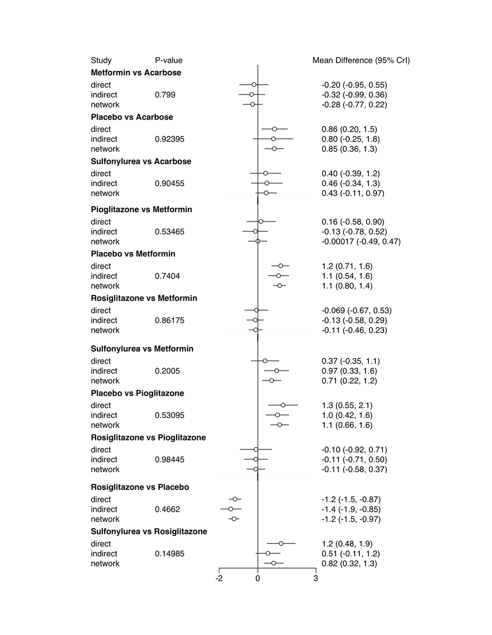
11.2.4 Generating the network meta-analysis results
Now that we produced our network meta-analysis model, and have convinced ourselves of its appropriateness, it is time to finally produce the results of our analysis, which we can report in our research paper.
As said before, the main question we may want to answer in network meta-analysis is: which treatment performs the best? To answer this question, we might first use the rank.probability() function, which calculates the probability for each treatment to be the best, second best, third best, and so forth, option. We only have to plug our mcmc2 object into this function, and additionally specify the preferredDirection. If smaller (i.e. negative) effect sizes indicate better outcomes, we set preferredDirection=-1, otherwise we use preferredDirection=1. We save the result of the function as rank, and then plot the results in a so-called rankogram.
rank <- rank.probability(mcmc2, preferredDirection = -1)
plot(rank, beside=TRUE, cex.names=0.5)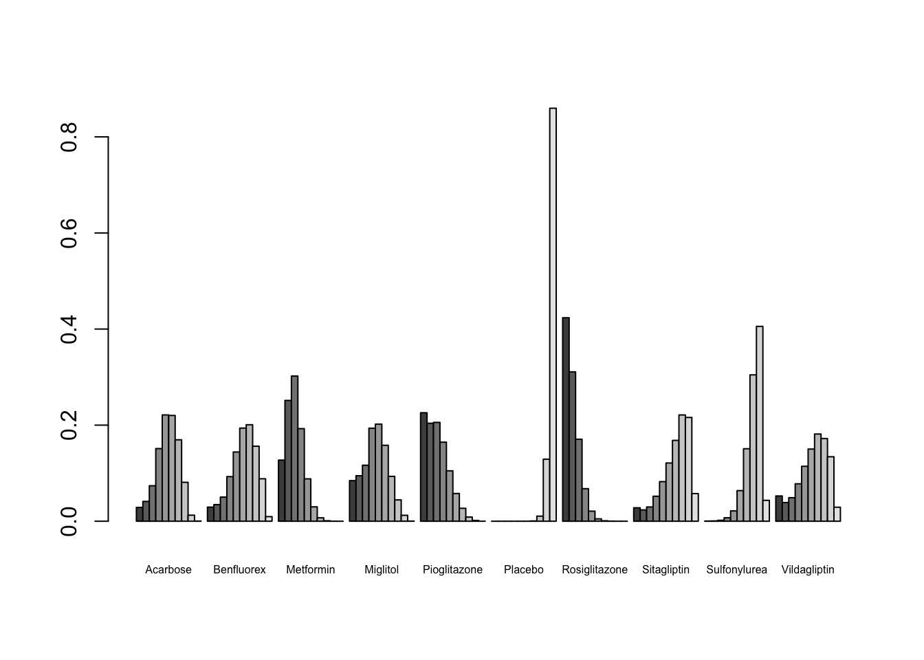
According to this plot, we see that Rosiglitazone may probably be the best treatment option under study, given that its first bar (signifying the first rank) is the largest. This finding is in agreement with the results from the frequentist analysis, where we found the same pattern.
Additionally, we can also produce a forest plot of our results using the forest() function. To do this, we first have to put our results object into the relative.effect() function and have to specify t1, the reference treatment. Then, we plug this into the forest() function to generate the plot.
forest(relative.effect(mcmc2, t1 = "Placebo"))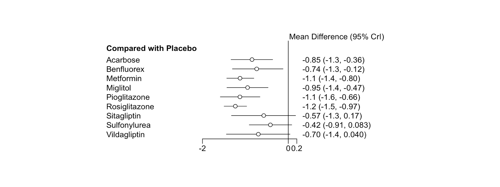
In the chapter on frequentist network meta-analysis, we already covered the P-score as a metric to evaluate which treatment in a network is likely to be the most efficacious. An equivalent to the P-score is the Surface Under the Cumulative RAnking (SUCRA) score, which can be calculated like this (Salanti, Ades, and Ioannidis 2011):
\[ SUCRA_j = \frac{\sum_{b=1}^{a-1}cum_{jb}}{a-1}\]
Where \(j\) is some treatment, \(a\) are all competing treatments, \(b\) are the \(b = 1, 2, ... a-1\) best treatments, and \(cum\) represents the cumulative probability of a treatment being among the \(b\) best treatments. To do this, we prepared the sucra function for you. The sucra function is part of the dmetar package. If you have the package installed already, you have to load it into your library first.
library(dmetar)If you don’t want to use the dmetar package, you can find the source code for this function here. In this case, R doesn’t know this function yet, so we have to let R learn it by copying and pasting the code in its entirety into the console in the bottom left pane of RStudio, and then hit Enter ⏎. The function then requires the ggplot2 and forcats package to work.
The function only needs a rank.probability() object as input, and we need to specify if lower values indicate better outcomes in our context by specifying lower.is.better. Let us see what results we get.
rank.probability <- rank.probability(mcmc2)
sucra(rank.probability, lower.is.better = TRUE)
Figure 11.1: SUCRA Score
Looking at the SUCRA values of each treatment, we again see that Rosiglitazone may be the best treatment, followed by, with some distance, Metformin and Pioglitazone.
A last thing we also often want to report in our research paper is the effect size estimate for each treatment comparison, based on our model. We can easily export such a matrix using the relative.effect.table() function. We can save the results of this function in an object, such as result, which we can then save to .csv file for later usage. The relative.effect.table() automatically creates a treatment comparison matrix containing the estimated effect, as well as the credibility intervals for each comparison. Here is how we can do this:
results <- relative.effect.table(mcmc2)
save(results, file = "results.csv")
11.2.5 Network Meta-Regression
One big asset of the gemtc package is that it allows us to conduct network meta-regressions. Much like conventional meta-regression (see Chapter 8), we can use this functionality to determine if specific study characteristics influence the magnitude of effect sizes found in our network. It can also be a helpful tool to check if controlling, for example, for methodological differences between the studies, leads to less inconsistency in our estimates.
Let us assume that in our network meta-analysis, we want to check if the Risk of Bias of a study has an influence on the effect sizes. For example, it could be the case that studies with a high risk of bias generally report higher effects compared to the control group or the alternative treatment. By including risk of bias as a covariate, we can control for this and check if risk of bias affects the effect sizes.
The procedure for a network meta-regression is largely similar to the one for a normal network meta-analysis. We start by generating a mtc.network object. To do this, we again use our data dataset. However, for a network meta-regression, we need to prepare a second dataframe in which information on the covariate we want to analyse is stored. I called this dataframe studies.df. It contains one column study with the name of each included study, and another column low.rob, in which it is specified if the study received a low risk of bias rating or not. For the second column, we used a binary coding scheme, in which 0 refers to high, and 1 to low risk of bias. If you analyze a categorical predictor, your subgroup codes must follow this scheme. For a continuous covariate, one can simply use the value each study has on the covariate. Here is my studies.df dataframe:
We can now define the network using the mtc.network function. We provide the function with the dataframe containing the effect sizes, and the study and covariate dataframe (argument studies). We save the output as network.mr.
network.mr <- mtc.network(data.re = data,
                          studies = studies.df)
Now, we can define the regressor we want to include in our network meta-analysis model. This can be done by generating a list object with three elements:
coefficient: We set this element to'shared', because we want to estimate one shared coefficient for the effect of (low) risk of bias across all treatments included in our network meta-analysis.variable: Here, we specify the name of the variable we want to use as the covariate (in this case,low.rob).control: We also have to specify the treatment which we want to use as the control against which the other treatments are compared.
regressor <- list(coefficient = 'shared',
                  variable = 'low.rob',
                  control = 'Placebo')
Next, we can define the model we want to fit. We provide the mtc.model function with the network we just generated, set the type of our model to "regression", and provide the function with the regressor object we just generated (argument regressor). We save the output as model.mr.
model.mr <- mtc.model(network.mr,
                      type = "regression",
                      regressor = regressor)
After this step, we can proceed to estimating the model parameters via the Markov Chain Monte Carlo algorithm using the mtc.run function. We use the same specifications as in the mcmc2 model. The results are saved as mcmc3.
mcmc3 <- mtc.run(model.mr,
                 n.adapt = 5000,
                 n.iter = 100000,
                 thin = 10)
We can analyze the results by pluggin the mcmc3 object into the summary function.
summary(mcmc3)##
## Results on the Mean Difference scale
##
## Iterations = 5010:105000
## Thinning interval = 10
## Number of chains = 4
## Sample size per chain = 10000
##
## 1. Empirical mean and standard deviation for each variable,
## plus standard error of the mean:
##
## Mean SD Naive SE Time-series SE
## d.Acarbose.Metformin -0.2550 0.25022 0.0012511 0.0013956
## d.Acarbose.Placebo 0.9124 0.25246 0.0012623 0.0015223
## d.Acarbose.Sulfonylurea 0.4393 0.27210 0.0013605 0.0014474
## d.Placebo.Benfluorex -0.7001 0.30124 0.0015062 0.0015125
## d.Placebo.Miglitol -0.9843 0.24290 0.0012145 0.0012679
## d.Placebo.Pioglitazone -1.1230 0.22810 0.0011405 0.0011627
## d.Placebo.Rosiglitazone -1.2891 0.14457 0.0007229 0.0008273
## d.Placebo.Sitagliptin -0.4604 0.38496 0.0019248 0.0020539
## d.Placebo.Vildagliptin -0.5917 0.38651 0.0019326 0.0020943
## sd.d 0.3378 0.08167 0.0004084 0.0004539
## B -0.2165 0.21542 0.0010771 0.0018536
##
## 2. Quantiles for each variable:
##
## 2.5% 25% 50% 75% 97.5%
## d.Acarbose.Metformin -0.74457 -0.4176 -0.2556 -0.09424 0.24254
## d.Acarbose.Placebo 0.40548 0.7500 0.9155 1.07845 1.40432
## d.Acarbose.Sulfonylurea -0.09859 0.2640 0.4385 0.61476 0.98296
## d.Placebo.Benfluorex -1.28585 -0.8985 -0.7034 -0.50702 -0.09316
## d.Placebo.Miglitol -1.46437 -1.1426 -0.9857 -0.82583 -0.50151
## d.Placebo.Pioglitazone -1.56718 -1.2712 -1.1254 -0.97646 -0.66681
## d.Placebo.Rosiglitazone -1.57252 -1.3829 -1.2900 -1.19725 -0.99743
## d.Placebo.Sitagliptin -1.23163 -0.7024 -0.4597 -0.21619 0.30661
## d.Placebo.Vildagliptin -1.36367 -0.8363 -0.5893 -0.34414 0.17341
## sd.d 0.20951 0.2802 0.3274 0.38346 0.52662
## B -0.63783 -0.3563 -0.2183 -0.07750 0.21243
##
## -- Model fit (residual deviance):
##
## Dbar pD DIC
## 26.99830 12.45411 39.45241
##
## 27 data points, ratio 0.9999, I^2 = 4%
##
## -- Regression settings:
##
## Regression on "low.rob", shared coefficients, "Placebo" as control
## Input standardized: x' = (low.rob - 0.5) / 1
## Estimates at the centering value: low.rob = 0.5The results for our covariate are reported under B. Because of the binary (i.e. 0 and 1) coding scheme, the value reported for B represents the change in effects associated with a study having a low risk of bias. In the second table (Quantiles for each variable), we see that the median for low risk of bias is \(-0.2183\), and that the 95% Credibility Interval ranges from \(-0.64\) to \(0.21\), including zero. We can explore the effect size differences further by generating two forest plots for the relative effects of each treatment compared to placebo, separately for studies with a low vs. high risk of bias. We can do this by using the relative.effect function, and specifying the covariate value. As said before, 0 represents studies with a high, and 1 studies with a low risk of bias.
forest(relative.effect(mcmc3, t1 = "Placebo", covariate = 1))
forest(relative.effect(mcmc3, t1 = "Placebo", covariate = 0))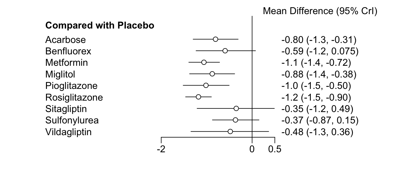
By comparing the forest plots, we can see that there is a pattern, with effects for low risk of bias studies being higher (i.e., more negative). This corresponds with the value B we found previously, although the credibility interval of this estimate does include zero.
Lastly, we can also examine if the network meta-regression model we generated fits the data more closely than the “normal” network meta-analysis model without the covariate we fitted before. To do this, we can compare the Deviance Information Criterion (\(DIC\)), which can be seen as an equivalent to the \(AIC\) or \(BIC\) typically used for conventional meta-regression. We can access the \(DIC\) of both the mcmc3 and mcmc2 model using this code.
summary(mcmc3)$DIC## Dbar pD DIC data points
## 26.99830 12.45411 39.45241 27.00000summary(mcmc2)$DIC## Dbar pD DIC data points
## 26.83238 22.72678 49.55916 27.00000We see from the output that the \(DIC\) of our meta-regression model (\(39.45\)) is lower than the one of our previous model which did not control for risk of bias (\(DIC = 49.56\)). Lower \(DIC\) values mean better fit. Given that the difference in \(DIC\)s is around ten, we can conclude that the mcmc3 model fits the data better than our previous model (a rough rule of thumb for when to consider a \(DIC\) difference as substantial can be found here).
11.2.6 Summary
This is the end of our short introduction into network meta-analysis and the netmeta and gemtc package. We have described the general idea behind network meta-analysis, the assumptions and caveats associated with it, two different statistical approaches through which network meta-analysis can be conducted, and how they are implemented in R. Still, we would like to stress that what we covered here is still only a rough overview of this metholodological approach. There are many other techniques and procedures helpful in generating robust evidence for decision-making from network meta-analysis, and we recommend to get acquainted with them. Here are two rather easily digestable literature recommendations you may find helpful for this endeavor:
- Efthimiou, O., Debray, T. P., van Valkenhoef, G., Trelle, S., Panayidou, K., Moons, K. G., … & GetReal Methods Review Group. (2016). GetReal in network meta‐analysis: a review of the methodology. Research synthesis methods, 7(3), 236-263. Link
- Dias, S., Ades, A. E., Welton, N. J., Jansen, J. P., & Sutton, A. J. (2018). Network meta-analysis for decision-making. Wiley & Sons. Link
References
Valkenhoef, Gert van, Guobing Lu, Bert de Brock, Hans Hillege, AE Ades, and Nicky J Welton. 2012. “Automating Network Meta-Analysis.” Research Synthesis Methods 3 (4). Wiley Online Library: 285–99.
Marsman, Maarten, Felix D Schönbrodt, Richard D Morey, Yuling Yao, Andrew Gelman, and Eric-Jan Wagenmakers. 2017. “A Bayesian Bird’s Eye View of ‘Replications of Important Results in Social Psychology’.” Royal Society Open Science 4 (1). The Royal Society Publishing: 160426.
McGrayne, Sharon Bertsch. 2011. The Theory That Would Not Die: How Bayes’ Rule Cracked the Enigma Code, Hunted down Russian Submarines, & Emerged Triumphant from Two Centuries of Controversy. Yale University Press.
Etz, Alexander. 2018. “Introduction to the Concept of Likelihood and Its Applications.” Advances in Methods and Practices in Psychological Science 1 (1). SAGE Publications Sage CA: Los Angeles, CA: 60–69.
Shim, Sung Ryul, Seong-Jang Kim, Jonghoo Lee, and Gerta Rücker. 2019. “Network Meta-Analysis: Application and Practice Using R Software.” Epidemiology and Health 41. Korean Society of Epidemiology: e2019013.
Dias, Sofia, Alex J Sutton, AE Ades, and Nicky J Welton. 2013. “Evidence Synthesis for Decision Making 2: A Generalized Linear Modeling Framework for Pairwise and Network Meta-Analysis of Randomized Controlled Trials.” Medical Decision Making 33 (5). Sage Publications Sage CA: Los Angeles, CA: 607–17.
Efthimiou, Orestis, Thomas PA Debray, Gert van Valkenhoef, Sven Trelle, Klea Panayidou, Karel GM Moons, Johannes B Reitsma, Aijing Shang, Georgia Salanti, and GetReal Methods Review Group. 2016. “GetReal in Network Meta-Analysis: A Review of the Methodology.” Research Synthesis Methods 7 (3). Wiley Online Library: 236–63.
Salanti, Georgia, AE Ades, and John PA Ioannidis. 2011. “Graphical Methods and Numerical Summaries for Presenting Results from Multiple-Treatment Meta-Analysis: An Overview and Tutorial.” Journal of Clinical Epidemiology 64 (2). Elsevier: 163–71.
