7 Exercise 3: Transformation of the response and predicator

At times it will be necessary to transform both the response and the predictor. Using the SIMDATAST data set produce an ouput of your graphs in a 2 rows x 3 columns grid:
(a) i. Plot $y_1$ against $x_3$

2. Define the model for $y_1$ against $x_3$ and create the residual vs fitted values plot.

3. Log transform the response variable and produce a new scatterplot.

4. Define the model for $log(y_1)$ against $x_3$ and create a residual vs fitted values plot.

5. Square-root predictor and plot a scatterplot of $log(y_1)$ against $\sqrt{x_3}$

6. Define the model for $log(y_1)$ against $\sqrt{x_3}$ and create a residual vs fitted values plot.

# create 2 rows x 3 columns grid
par(mfrow = c(2, 3)) 

# plot y vs x3
plot(y1 ~ x3, data = SIMDATAST,main="Scatterplot of y1~x3") 
# define model for log transformed response y1 vs x3
mod1 <- lm(y1 ~ x3, data = SIMDATAST)
# you can choose to add the model line to the plot with abline(mod1)
# residual plot for mod1
plot(mod1, which = 1, main = "Residuals vs Fitted value for y1~x3")

# plot of log transformed y against x3
plot(log(y1) ~ x3, data = SIMDATAST, main = "Scatterplot of log(y1)~x3")
# define model for log transformed response y1 vs x3
mod2 <- lm(log(y1) ~ x3, data = SIMDATAST)
# optionally add abline(mod2) to the plot
# residual plot for mod2
plot(rstandard(mod2) ~ fitted(mod2), main="Residuals vs Fitted value for log(y1)~x3")
# optional to add abline(h=0,lty=3) to the plot

# plot of log transformed y against sqrt(x3)
plot(log(y1) ~ I(x3^0.5), data = SIMDATAST, main = "Scatterplot of log(y1)~sqrt(x3)")
mod3 <- lm(log(y1) ~ I(x3^.5), data = SIMDATAST) # define model for log transformed response y1 vs sqrt(x3)
#optional to add abline(mod3) to the plot
# residual plot for mod3
plot(rstandard(mod3) ~ fitted(mod3), main="Residuals vs fitted of log(y1)~sqrt(x3)")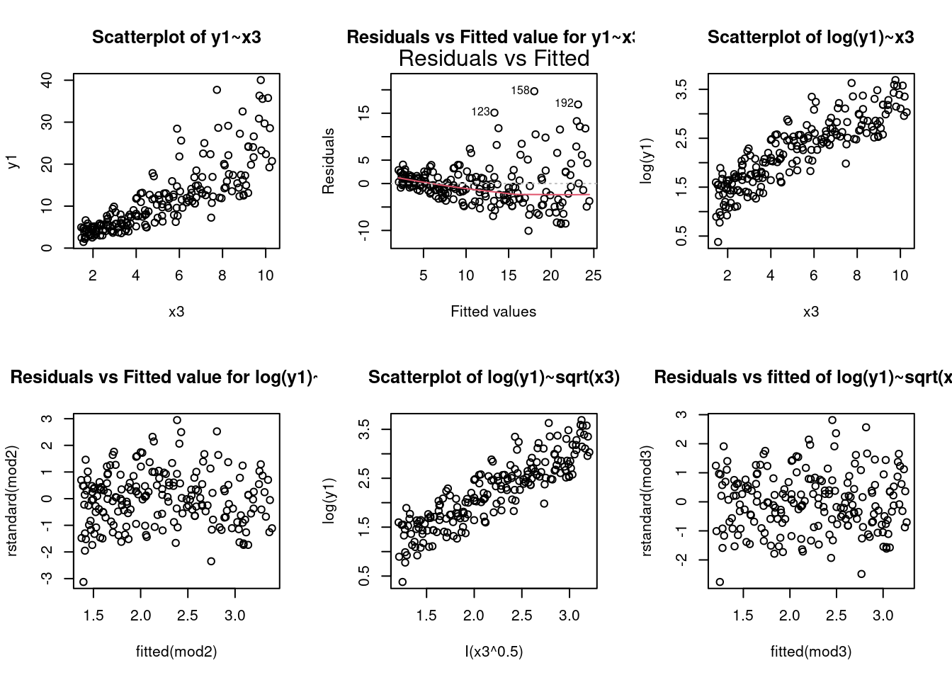

# optional to add abline(h=0,lty=3) to the plot