3 Example 2: Car stopping (power transformation on y)

The stopping.csv file contains 63 observations of cars. In these observations, two variables were recorded, namely the speed of cars when the brakes were applied (in mile per hour) and the stopping.

stopping <- read.csv("Stopping.csv")

(a) i. Create a scatterplot of Distance against Speed.

We can use the code plot(). What variables do we want on our x and y axis?

plot(Distance ~ Speed, data = stopping)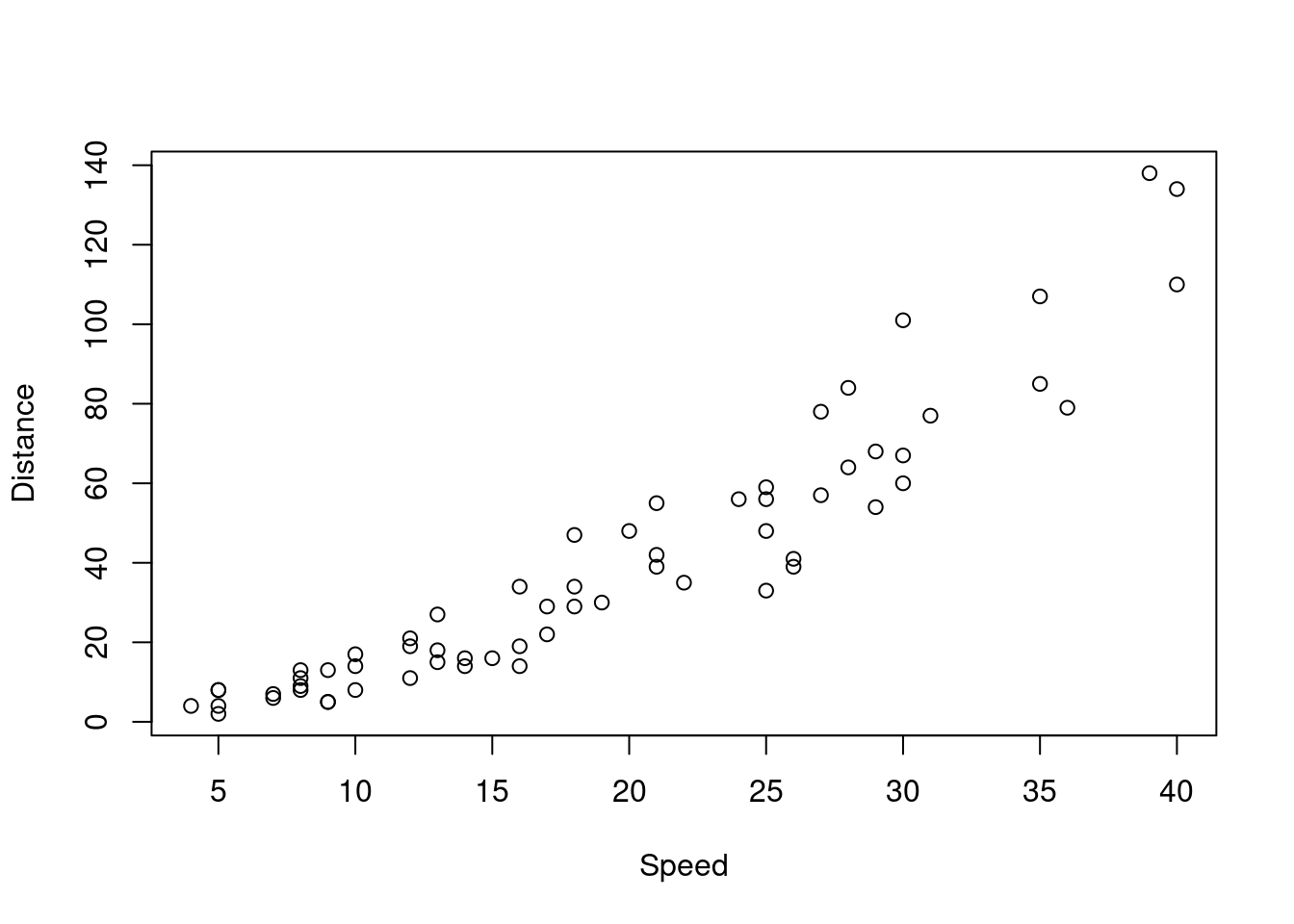

Look at your plot and pick the correct statement.

There is a no relationship between Stopping Distance and Speed There is an non-linear relationship between Stopping Distance and Speed and as Speed increases, Distance decreases TThere is an non-linear relationship between Stopping Distance and Speed and as Speed increases, Distance increases

As the relationship appears to be non-linear, we might want to apply a transformation to one of the variables.

What transformation should we apply here:
Create a new scatterplot of with the transformed data:

We can use the codeplot() again. Change Y to be the square root of your response variable. You may need to change the axis label too.

plot(sqrt(Distance) ~ Speed, data = stopping, ylab= "Square root of Distance (in feet)")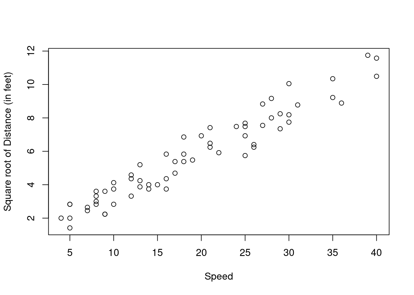

3.1 Statistical Analysis

The model for the relationship between Speed and sqrt(Distance) is therefore: \(\sqrt{Y_i} = \alpha + \beta x_i + \epsilon_i\), where \(\epsilon_i \sim N(0, \sigma^2)\) and \(i = 1, . . . , 63.\)

(b) What type of model is this?

Use the lm() function to fit this model to your plot: help(lm)

Use the help(lm) function to see what parameters you need within the function.

Model1 <- lm(sqrt(Distance) ~ Speed, data = stopping)

3.2 Assumption Checking

(c) i. Model assumptions can be assessed graphically by producing a plot of the residuals versus the fitted values and a normal probability plot (Q-Q plot) of the residuals.

Use the plot(rstandard()~fitted()) function for the residual plot and the code qqnorm for the Q-Q plot.

plot(rstandard(Model1) ~ fitted(Model1))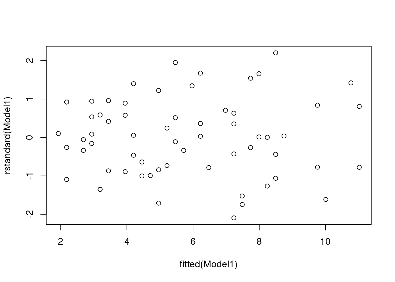

qqnorm(rstandard(Model1))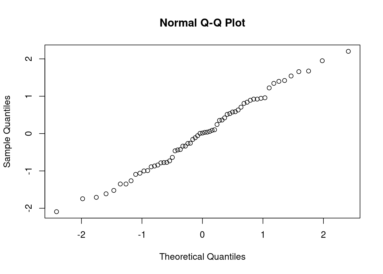

The residual vs fitted values plot shows that the points fairly evenly scattered above and below the, which suggests it reasonable to assume that the random errors have mean equal to .
In the normal probability plot, we see that points exactly lie on diagonal line. This indicates that the Normality assumption be satisfied. This is not ideal but, on the positive side, the estimates of parameters will not be affected and hence we can still use the model to describe the relationship between variables and make predictions.

3.3 Regression output

(d) i. Load the summary statistics:

summary(Model1)

## 
## Call:
## lm(formula = sqrt(Distance) ~ Speed, data = stopping)
## 
## Residuals:
##     Min      1Q  Median      3Q     Max 
## -1.4879 -0.5487  0.0098  0.5291  1.5545 
## 
## Coefficients:
##             Estimate Std. Error t value Pr(>|t|)    
## (Intercept) 0.918283   0.197406   4.652 1.82e-05 ***
## Speed       0.252568   0.009246  27.317  < 2e-16 ***
## ---
## Signif. codes:  0 '***' 0.001 '**' 0.01 '*' 0.05 '.' 0.1 ' ' 1
## 
## Residual standard error: 0.7193 on 61 degrees of freedom
## Multiple R-squared:  0.9244, Adjusted R-squared:  0.9232 
## F-statistic: 746.2 on 1 and 61 DF,  p-value: < 2.2e-16

Fill in the blanks in the regression equation with the calculated parameters to 3 decimal places:

\(\sqrt{Distance}\) = − \(\bigg(\) \(\cdot\) Speed \(\bigg)\)

Interpret the parameters correctly and enter any numbers to 2 decimal places:

This means the square root of distance is linearly related to speed. That is, as the speed increases by 1 MPH, the expected square root of distance by feet.

Using the created model predict the Stopping Distance if the Speed is 20MPH, to 2 decimal places:

When predicting the value of the response for a new observation, we need to back transform the transformed variable.

\(Distance = \bigg(\) + ( \(\cdot\) ) \(\bigg) ^2\) = feet.