6 Exercise 2

6.1 Exercise 2 part 1 - Transforming Y with ln

Note that the default understanding of log in R is $log_e$ = ln = log.

(a) Perform analysis the data frame SIMDATAST to create and display six graphs using a 2 by 3 layout.

1. Produce a scatterplot of $y_1$ versus $x_1$.

# Begin by setting up the 2x3 grid
par(mfrow = c(2, 3))
# Plot y1 vs x1
plot(y1 ~ x1, data = SIMDATAST)

2. Plot the residuals versus fits for the model created by regressing $y_1$ on $x_1$ (call this model modx1). Based on the first two graphs, does a logarithmic transformation for the response variable make sense?

# Define the model
modx1 <- lm(y1 ~ x1, data = SIMDATAST)
# Plot the residual graphs
plot(modx1, which = c(1,2))
#This plot function will produce many analytical graphs so using c(1,2) selects that you want the fitted residual plot and the Q-Q plot as they are the first 2 it produces.

(iii) In the second row of graphs, create a scatterplot of $ln(y_1$) versus $x_1$.

# Plot y1 vs ln(x1)
plot(log(y1) ~ x1, data = SIMDATAST)

(iv) Create a plot of the residuals versus the fits for the model and the Q-Q normal plot for log($y_1$) ~ $x_1$.

# Use the plot function: 
plot(lm(log(y1) ~ x1, data = SIMDATAST), which = c(1,2))
# when Par is run along with the rest of this code it will put the 6 graphs in the grid.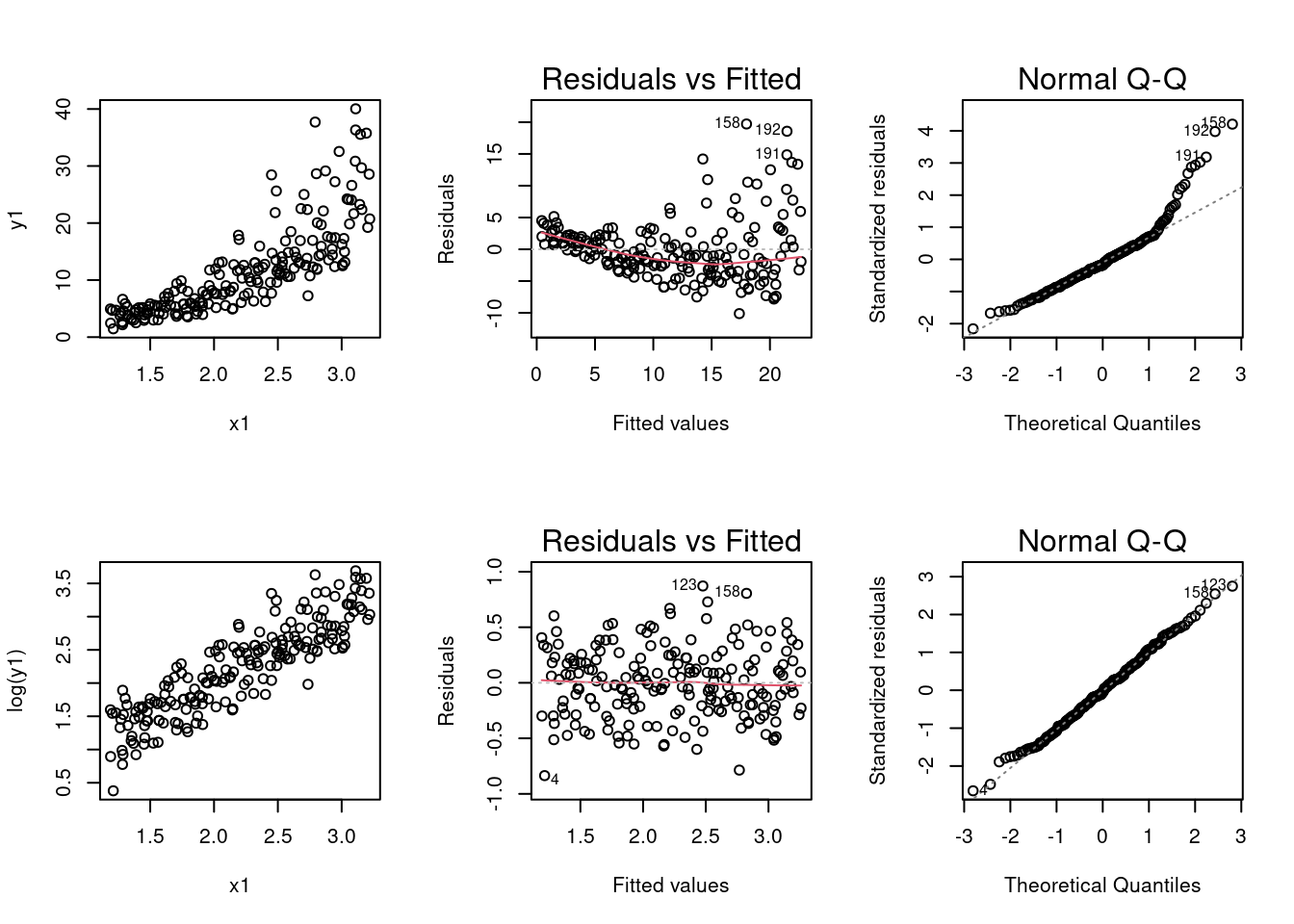

22. Based on the second row of graphs, do the assumptions for the normal error model seem to be satisfied for the model log($y_1$) ~ $x_1$? YesNo

6.2 Exercise 2 part 2 - Transforming Y with a reciprical

(a) Perform analysis the data frame SIMDATAST to create and display six graphs using a 2 by 3 layout.

1. Produce a scatterplot of $y_2$ versus $x_2$.

# Begin by setting up the 2x3 grid
par(mfrow = c(2, 3))
# Plot y1 vs x1
plot(y2 ~ x2, data = SIMDATAST)

2. Plot the residuals versus fits for the model created by regressing $y_2$ on $x_2$ (call this model modx2).

# Define the model
modx2 <- lm(y2 ~ x2, data = SIMDATAST)
# Plot the residual graphs
plot(modx2, which = c(1,2))
#This plot function will produce many analytical graphs so using c(1,2) selects that you want the fitted residual plot and the Q-Q plot as they are the first 2 it produces.

3. Based on the first two graphs, does a reciprocal transformation for the response variable make sense? YesNo
   

4. In the second row of graphs, create a scatterplot of $y_2^{-1}$ versus$x_2$.

# Plot y1 vs ln(x1)
plot((y2)^-1 ~ x2, data = SIMDATAST)

22. Create a plot of the residuals versus the fits and the Q-Q normal plot for $y_2^{-1} \sim x_2$.

# Use the plot function: 
plot(lm((y2)^-1 ~ x2, data = SIMDATAST), which = c(1,2))
# when Par is run along with the rest of this code it will put the 6 graphs in the grid.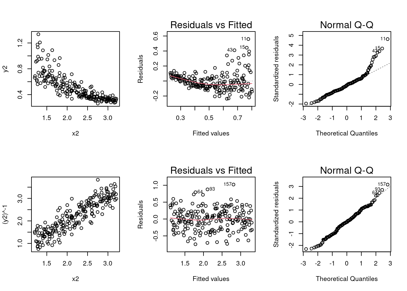

6. Based on the second row of graphs, do the assumptions for the normal error model seem to be satisfied for the model $y_2^{-1} \sim x_2$? YesNo