2 Example 1 - life expectancy (log-transformation on x)

Rossman (1994) collected information on life expectancy in various countries of the world and the densities of people per television set and of people per physician in those countries.

The data is available in the LifeExp.csv file. Remember you may need to reset your working directory and your data should be saved into that directory.

life <- read.csv("LifeExp.csv")

In this practical, our focus is to identify how female life expectancy (Y , abbreviated to FLE) is related to the number of people per physician (x, abbreviated to PPP).

(a) i. Create a scatterplot of FLE against PPP.

We can use the codeplot(). What variables do we want on our x and y axis?

plot(FLE ~ PPP, data = life)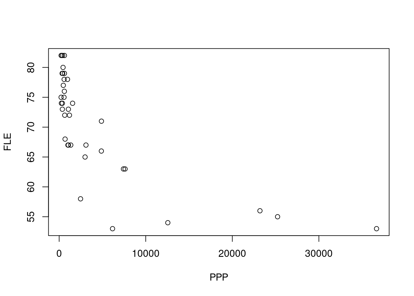

2. Look at your plot and pick the correct statement.

There is no relationship between Female Life Expectancy and People per Phyisician There is an inverse relationship between Female Life Expectancy and People per Phyisician and as PPP increases, FLE decreases There is an inverse relationship between Female Life Expectancy and People per Phyisician and as PPP increases FLE increases

As the relationship appears to be non-linear, we might want to apply a transformation to the predictor variable. Transforming the values of x might be the first thing to try if there is a non-linear monotonic (i.e. entirely non-increasing or entirely non-decreasing) trend in the data, and non-linearity is the only problem (i.e the model assumptions: independence, zero-mean, constant variance and normality should be met).

3. What transformation should we apply here: LogarithmicSquare-rootNo transformation
   

4. Create a new scatterplot of female life expectancy against the transformed PPP variable:

We can use the codeplot() again. Change x to be the log of your predictor variable. You may need to change the axis label too.

plot(FLE ~ log(PPP), data = life, xlab = "log(PPP)")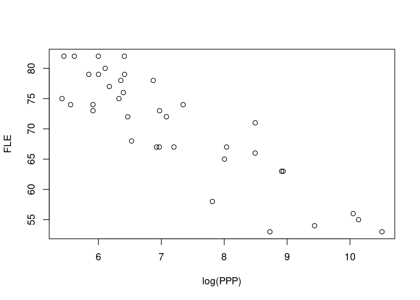

2.1 Statistical Analysis

The model for the relationship between FLE and log(PPE) is therefore: \(Y_i = \alpha + \beta \cdot log(x_i) + \epsilon_i\), where \(\epsilon_i \sim N(0, \sigma^2)\) and \(i = 1, . . . , 37.\)

(b) What type of model is this? Simple Linear RegressionMultiple RegressionNon-linear Regression

1. Use the lm() function to fit this model to your plot: help(lm)

Use the help(lm) function to see what parameters you need within the function.

Model1 <- lm(FLE ~ log(PPP), data = life)

2.2 Assumption Checking

(c) i. Model assumptions can be assessed graphically by producing a plot of the residuals versus the fitted values and a normal probability plot (Q-Q plot) of the residuals.

Use the plot(rstandard()~fitted()) function for the residual plot and the code qqnorm for the Q-Q plot.

plot(rstandard(Model1) ~ fitted(Model1))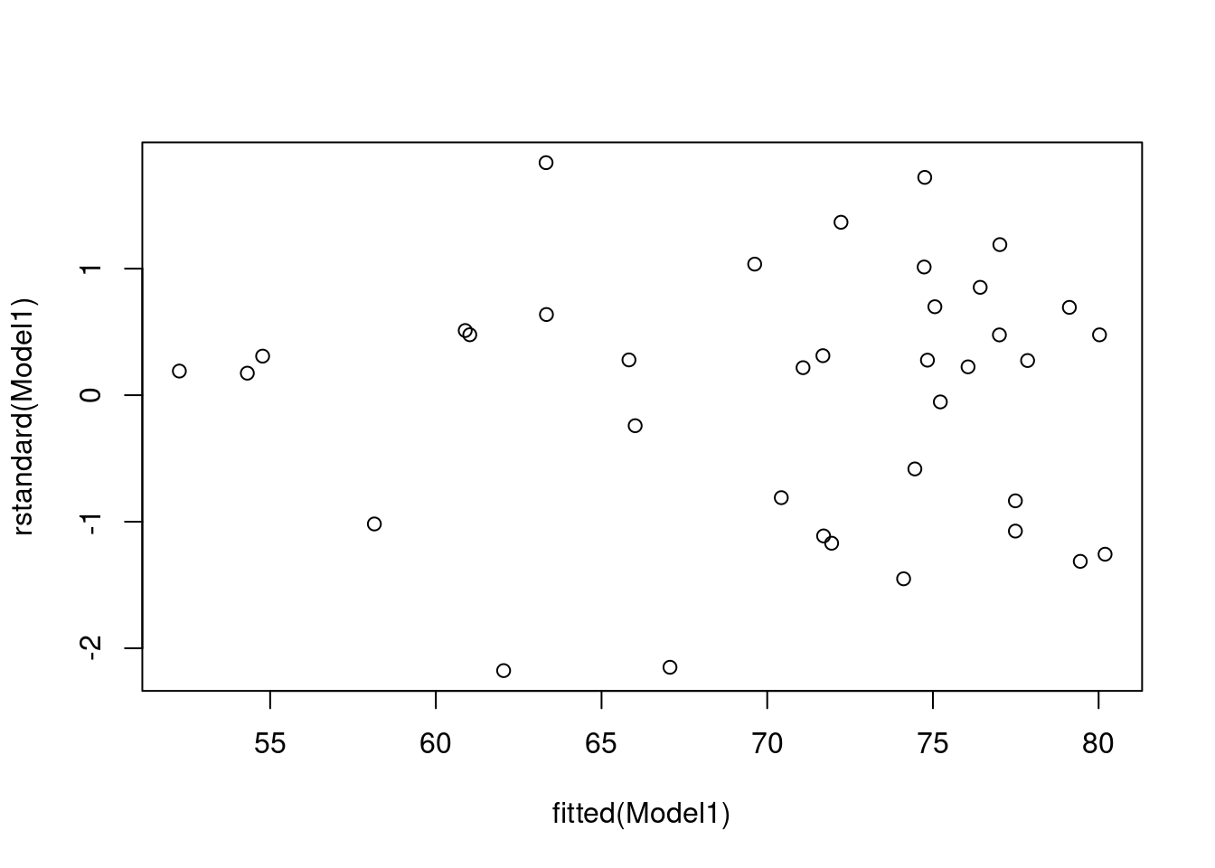

qqnorm(rstandard(Model1))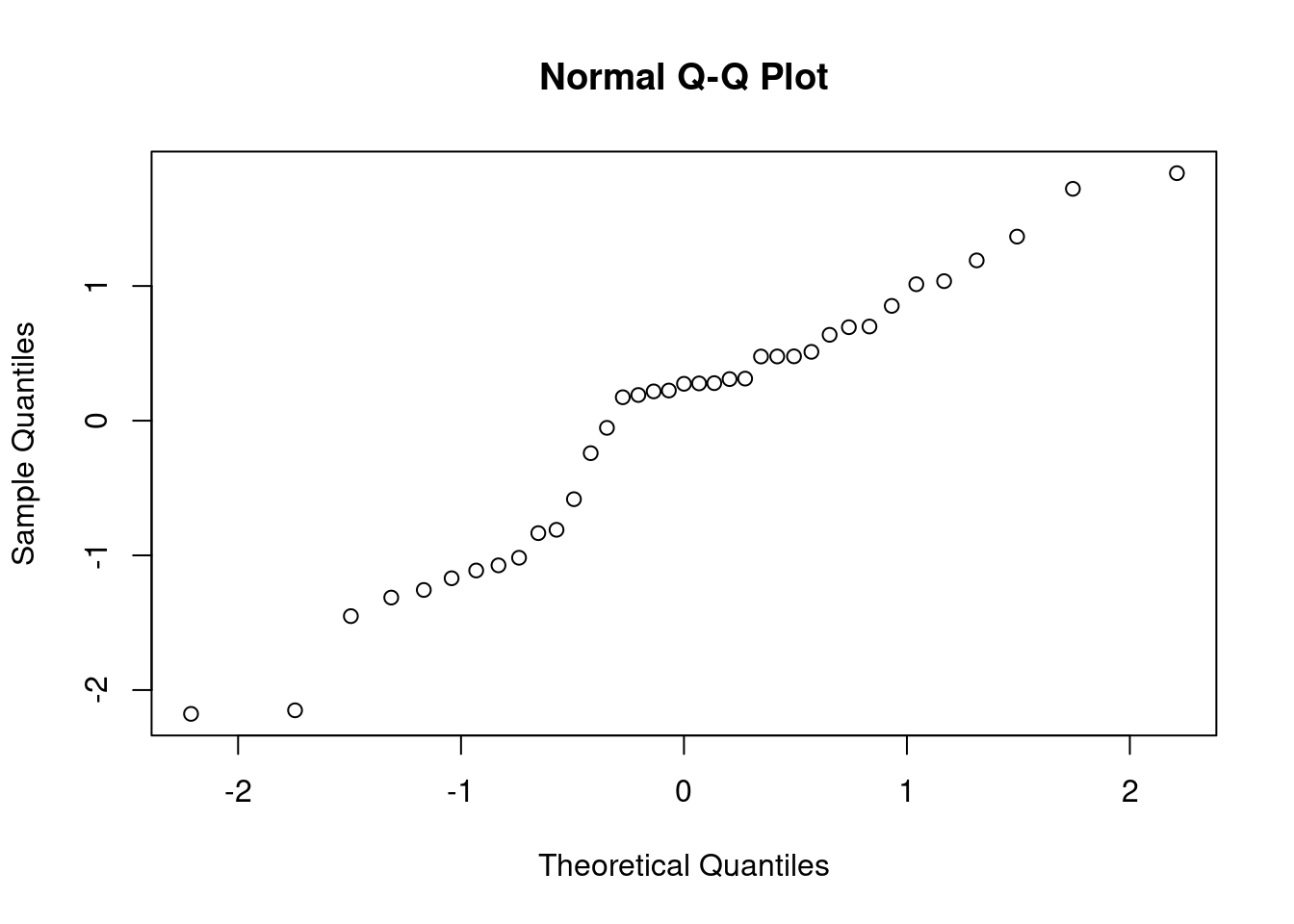

2. The residual vs fitted values plot shows that the points areare not fairly evenly scattered above and below themean linezero line, which suggests it isis not reasonable to assume that the random errors have mean equal to µzero. The vertical variation of the points seems to be small for small fitted values. However, there are also fewer points in this case. It would be preferable if moreless data were available.
   

3. In the normal probability plot, we see that points dodo not exactly lie on diagonal line. This indicates that the Normality assumption maymay notbe satisfied.
   

4. The independence of the random errors seemsdoes not seem reasonable since each point refers to a different country.

2.3 Regression output

(d) i. Load the summary statistics:

summary(Model1)

## 
## Call:
## lm(formula = FLE ~ log(PPP), data = life)
## 
## Residuals:
##    Min     1Q Median     3Q    Max 
## -9.065 -3.489  1.143  2.663  7.674 
## 
## Coefficients:
##             Estimate Std. Error t value Pr(>|t|)    
## (Intercept) 109.9498     3.6860   29.83  < 2e-16 ***
## log(PPP)     -5.4893     0.5036  -10.90 8.48e-13 ***
## ---
## Signif. codes:  0 '***' 0.001 '**' 0.01 '*' 0.05 '.' 0.1 ' ' 1
## 
## Residual standard error: 4.286 on 35 degrees of freedom
## Multiple R-squared:  0.7724, Adjusted R-squared:  0.7659 
## F-statistic: 118.8 on 1 and 35 DF,  p-value: 8.484e-13

2. Fill in the blanks in the regression equation with the calculated parameters to 2 decimal places:

\(FLE\) = − \(\bigg(\) \(\cdot\) \(log(PPP)\bigg)\)

3. Interpret the parameters correctly and enter any numbers to 2 decimal places:

This means the female life expectancy is seemsdoes not seem related to the number of people per physician. If log(PPP) increases by 1 unit, the expected female life expectancy increasesdecreases by .

4. Using the created model predict the life expectancy if the number of people per physician is 4000, to 2 decimal places:

When predicting the value of the response for a new observation, we need to back transform the variable.

\(FLE\) = − \(\bigg(\) \(\cdot\) \(log(\)\()\bigg)\) =