Ordinary Differential Equation Modelling with ‘ecode’

4.1 Phase Curve

Numerical solutions are often used to explore complex ODEs. Simulations start with an initial condition x(0) at time t = 0. For each small time interval Δt, simulation proceeds by

\[ x(t + Δt) = x(t) + dx/dt · Δt \]

In ‘ecode’, simulations can be performed using the function eode_proj(),

eq1 <- function(x, y, r1 = 4, a11 = 1, a12 = 2) (r1 - a11 * x - a12 * y) * x
eq2 <- function(x, y, r2 = 1, a21 = 2, a22 = 1) (r2 - a21 * x - a22 * y) * y
x <- eode(dxdt = eq1, dydt = eq2, constraint = c("x<1","y<1"))
pc <- eode_proj(x, value0 = pp(list(x = 0.2, y = 0.1)), N = 100, step = 0.01)

The first argument of the function eode_proj() specifies the ODE system under concern, the second argument being an object of ‘pp’ type that specifies the initial condition, the third argument being the number of iterations, and the last argument being time step Δt (default as 0.01).

The output of the function eode_proj() is an object of ‘pc’ type, short for ‘phase curve’. It records how the phase point moves over time until the last iteration. To visualise the object, simply use the plot() function. The result shows that species x reached its maximal population size at t = 0.5, or the 50th iteration (Figure 4.1).

plot(pc)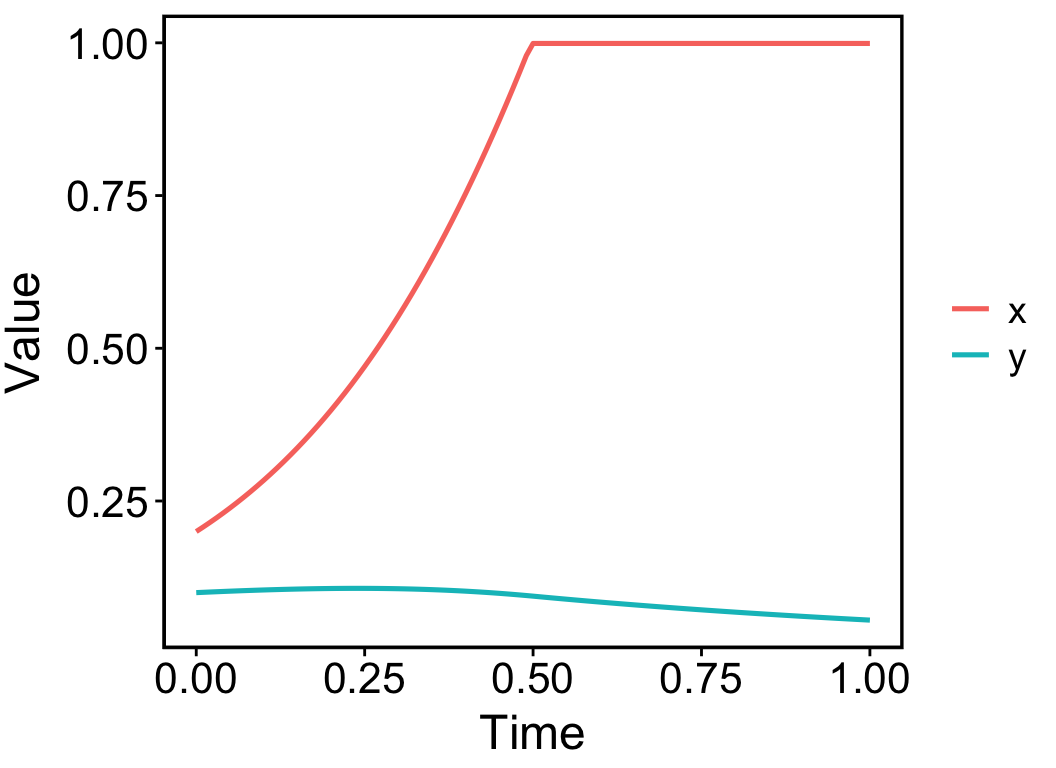

Figure 4.1: Simulation outputs of simple Lotka–Volterra competition equations. Given by the function plot() on ‘pc’ objects. Each line shows how a state variable changes over time.

Alternatively, the simulation output can be visualised in a phase plane using the function pc_plot(). The result is shown in Figure 4.2.

pc_plot(pc)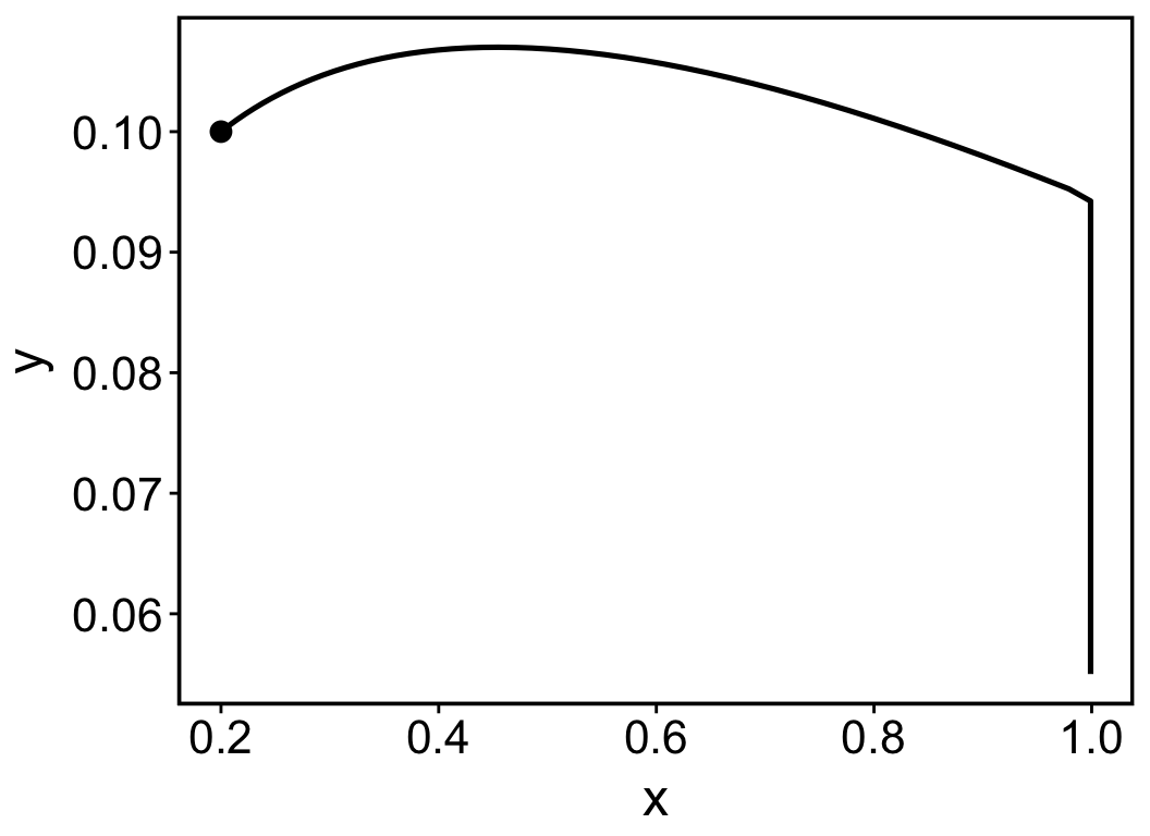

Figure 4.2: Phase curve of simple Lotka–Volterra competition equations with an initial condition of x(0) = 0.2, y(0) = 0.1. Given by the function pc_plot() on ‘pc’ objects. The solid point represents the initial state of the system. The phase point moves from the solid point to the other end of the curve during the simulation.

4.2 Variable Calculator

Sometimes, we are interested in other quantities aside from state variables. For example, we may want to calculate the total individuals of all species, rather than the population size of species x or y. In this case, we wish to define a new variable z = x + y, and track how variable z changes over time.

eq1 <- function(x, y, r1 = 4, a11 = 1, a12 = 2) (r1 - a11 * x - a12 * y) * x
eq2 <- function(x, y, r2 = 1, a21 = 2, a22 = 1) (r2 - a21 * x - a22 * y) * y
x <- eode(dxdt = eq1, dydt = eq2, constraint = c("x<100","y<100"))
pc <- eode_proj(x, value0 = pp(list(x = 0.2, y = 0.1)), N = 100)
pc_new <- pc_calculator(pc, formula = "z = x + y")

plot(pc_new)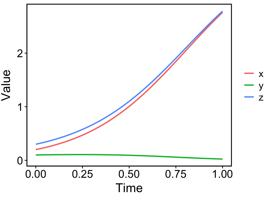

Figure 4.3: Track the total number of individuals of all species by defining a new variable z = x + y. Achieved by the function pc_calculator(), and visualised by the function plot() on ‘pc’ objects.

The function pc_calculator() helps to calculate new variables with specified formulas. It returns a new ‘pc’ object that can be plotted by the plot() function. The argument ‘formula’ supports any calculations on state variables and model parameters. For example, the following code tracks how the velocity vector of variable x changes over time,

pc_new <- pc_calculator(pc, formula = "dxdt = (r1 - a11 * x - a12 * y) * x")
plot(pc_new)

This formula will be interpreted as that state variables x, y change over time, but model parameters \(r_1\), \(a_{11}\), and \(a_{12}\) are constant.

4.3 Sensitivity

Sensitivity analysis helps to explore whether model predictions are sensitive to changes in model parameters or initial conditions. Simulations are often repeatedly performed with different values of parameters or initial conditions.

eq1 <- function(x, y, r1 = 4, a11 = 1, a12 = 2) (r1 - a11 * x - a12 * y) * x
eq2 <- function(x, y, r2 = 1, a21 = 2, a22 = 1) (r2 - a21 * x - a22 * y) * y
x <- eode(dxdt = eq1, dydt = eq2, constraint = c("x<100","y<100"))
res <- eode_sensitivity_proj(x, valueSpace = list(x = c(0.2, 0.3, 0.4), y = 0.1, a11 = 1:3), N=100, step = 0.01)

The function eode_sensitivity_proj() gives a handy way to perform repeated simulations. The second argument valueSpace should be a list. Each component of the list specifies possible values of a model parameter or initial values of a state variable. The above code will end up performing 3×1×3 = 9 simulations. The function returns an object of ‘pcfamily’, short for ‘a family of phase curves’. It can also be visualised by plot() function to see how projected curves change with different settings and scenarios.