1 Basic Concepts in Ordinary Differential Equations
1.1 System
Ordinary Differential Equations (ODEs) is widely used to study the evolution of a system. A system can be any collection of parts that interact with each other, functioning as a whole. An ecosystem has plants, animals, microbes, and the physical environment. They interact with each other by positively or negatively affecting the growth of each population or resource availability. The global climate system is made up of five parts: atmosphere, lithosphere, hydrosphere, cryosphere, and biosphere. The state of climate is influenced by many factors in its parts. When we say the evolution of a system, we mean how the system changes over time.
It is impossible to model all features of a system and, therefore, a full depiction of system evolution is unfeasible. The state of a system at a particular time is often approximated by a set of state variables. For example, in a wolf–sheep system, two fundamental variables are the number of wolves and sheep, although other variables, such as grass availability, could also be added. The goal of an ODE could be to track how wolves and sheep populations change over time.
We could then describe system dynamics using ODEs,
dx/dt = v(x)
where x = (x1, x2, … xn)T is a vector of system variables x1, x2, … xn, v(x) the velocity of these variables as a function of the variable themselves. The velocity function vi(x) (i = 1, 2, …, n) determines how variable xi changes at a particular state (x1, x2, … xn)T. Positive velocity results in a growth of xi, and the value of velocity indicates the speed of change.
1.2 Phase Plane
The state of a system changes from time to time. To present differential equations visually, a system is considered to be a phase point moving inside a n-dimensional space. A phase point is the values of system variables at a particular time. At time t, it can be mathematically described as x(t) = (x1(t), x2(t), … xn(t))T. The initial state of the system at time t0 = 0 is thus approximated by the phase point x(t0) = (x1(t0), x2(t0), … xn(t0))T. For example, a wolf–sheep system has 100 wolves and 300 sheep initially if x(0) = (100, 300)T.
A phase plane is a n-dimensional space, containing all possible values of phase points. The wolf–sheep system has a 2-dimensional phase plane, each axis being the number of wolves and sheep. Phase points are allowed to move inside the phase plane, forming a trajectory called phase curve (or phase line). For an autonomous ordinary differential equation (see definition in Section 1.3), a phase curve is uniquely determined by the equations and the initial conditions. In other words, with a fixed initial state and interaction rules, the phase point of a system behaves the same. Meanwhile, phase curves are visual presentations of the solutions of differential equations. When ODEs could not be solved analytically, it is a good practice to visualise system behaviours in this way.
Every phase point is attached with a phase velocity vector, which defines how the point will move in the next time step. Phase velocity vector is the value of v(x) at a particular phase point. For a 1-dimensional ODE,
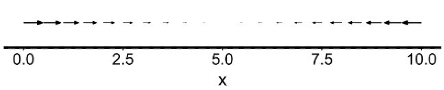
dx/dt = 25 - 5x (0<x<10)
The phase velocity vector is v(x) = 25 – 5x. When x is larger than 5, the velocity goes negative and thus the quantity of x is expected to decrease. The larger the x is, the faster it will decrease. When x equals to 5, the velocity becomes 0, indicating that x will no longer move. This point is called an equilibrium, as the system will ultimately converge to this point irrespective of its initial condition.
As shown in Figure 1.1, a collection of phase velocity vectors in the phase plane is a phase velocity vector field. The movement of a phase point will always follow a route defined by the phase velocity vector field. For example, objects of all kinds will ultimately hit the ground if gravity is the only force acting upon it. Electrically charged particles will always be forced by electric fields created by other particles.
1.3 Autonomous system
A system is called autonomous if the movement of phase point is only dependent on itself. In other words, the phase velocity vector v(x) is a function of x itself. Analytical methods such as equilibrium and stability require the system to be autonomous (See Chapter 3), while a non-autonomous system may be too complex to analyse its convergence behaviour. In reality, however, a natural population is often forced by external variables such as the climate. These variables are not affected by system states, but are able to drive system changes, sometimes even substantial such as the transition between tropical forests and savanna. Ecosystems are thus often non-autonomous, but can be simplified to autonomous systems to find general theories if this assumption does not affect the main conclusion. It is up to the researchers to choose an appropriate model for accuracy prediction or exploratory analysis. In package ‘ecode’, stability and equilibrium modules (Chapter 3) are available for autonomous systems. Numerical simulations can apply for both autonomous and non-autonomous ones (Chapter 4).