eq1 <- function(x, y, r1 = 1, a11 = 1, a12 = 2) (r1 - a11 * x - a12 * y) * x
eq2 <- function(x, y, r2 = 1, a21 = 2, a22 = 1) (r2 - a21 * x - a22 * y) * y
x <- eode(dxdt = eq1, dydt = eq2)
eode_get_cripoi(x, init_value = pp(list(x = 0.5, y = 0.5)))
## phase point:
## x = 0.3333333
## y = 0.33333333 Analytical Methods
3.1 Equilibrium
In ‘ecode’, any phase point is presented by an object of ‘pp’ type. Constructor function pp() can be used to create an object of phase point. For example, the code pp(list(x = 1, y = 1)) returns a phase point object that is featured with two state variables x and y, whose values are 1.
Equilibrium point is a special phase point that lets the phase velocity vector be zero,
\[ dx^*/dt = v(x^*) = 0 \]
Equilibrium point x* can be obtained by solving n equations of n variables. Package ‘ecode’ uses Newton iteration method to get an approximate solution of x*,
\[ x_{n+1} = x_n – J^{–1}(x_n)v(x_n) \]
where matrix J(x) is the Jacobian matrix of the multivariate function v(x),
\[ J(\chi_{ij})~=~[\partial\nu_i/\partial\chi_j] \]
By specifying an initial phase point \(x_0\), the algorithm can iteratively approach the solution of the equation \(v(x^*) = 0\) when n becomes large. This can be achieved by the function eode_get_cripoi(),
The first argument of the function eode_get_cripoi() specifies the ODE system under concern, and the second argument specifies the initial phase point \(x_0\). The function returns a ‘pp’ object, the equilibrium point found. Different \(x_0\) can be explored to see if there are other equilibrium points, as searching paths vary substantially with different \(x_0\).
3.2 Stability
Stability is a key concern of any system. A phase point does not change at an equilibrium point, but it may not be the case when it locates at the neighbourhood of the equilibrium. If a phase point converges towards the equilibrium when it is perturbed at the equilibrium, the equilibrium point is called stable. If the phase point goes away under perturbation, the equilibrium point is called unstale. The stability of an equilibrium point is determined by linear approximation method. At an equilibrium point \(x^* = (x_1^*, x_2^*, …, x_n^*)\), the ODE system \(dx/dt = v(x)\) can be linearised as,
\[ \frac{dx_1}{dt}=\left(\frac{\partial v_1}{\partial x_1}\right)^\ast dx_1+\left(\frac{\partial v_1}{\partial x_2}\right)^\ast dx_2+...+\left(\frac{\partial v_1}{\partial x_n}\right)^\ast dx_n+O_1(x_1,x_2,\ ...,\ x_n) \]
\[ \frac{dx_2}{dt}=\left(\frac{\partial v_2}{\partial x_1}\right)^\ast dx_1+\left(\frac{\partial v_2}{\partial x_2}\right)^\ast dx_2+...+\left(\frac{\partial v_2}{\partial x_n}\right)^\ast dx_n+O_2(x_1,x_2,\ ...,\ x_n) \]
\[ ... \]
\[ \frac{dx_1}{dt}=\left(\frac{\partial v_n}{\partial x_1}\right)^\ast dx_1+\left(\frac{\partial v_n}{\partial x_2}\right)^\ast dx_2+...+\left(\frac{\partial v_n}{\partial x_n}\right)^\ast dx_n+O_n(x_1,x_2,\ ...,\ x_n) \]
where \((∂vi/∂x_j)\) is the partial derivative of vi with respect to xj, \((∂vi/∂x_j)^*\) the value of the partial derivative at the equilibrium point \(x^*, O(x_1, x_2, …, x_n)\) a small quantity that is negligible. Then, the stability of x* with respect to the linearised system (or the primitive system dx/dt = v(x)) is determined by the eigenvalues of the system matrix \(J = [(∂vi/∂x_j)^*]_{n×n}\). If all the eigenvalues \(λ_1, λ_2, …, λ_n\) are less than zero, the equilibrium point is stable. If any of the eigenvalues is larger than zero, the equilibrium point is unstable.
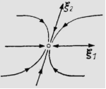
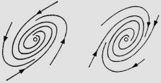
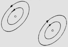
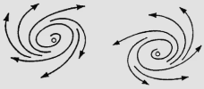
The eigenvalues can sometimes be complex numbers. The imagery part of eigenvalues leads to the result that a phase point approaches stable equilibria with spiral trajectory rather than approaching it directly. Similarly, it follows a spiral trajectory when going away from unstable equilibria. This phenomena leads to a conceptual distinction that stable points with eigenvalues being real numbers are called stable nodes, while stable points with complex eigenvalues are called stable foci. A full list of concepts are shown in Table 3.1.
| Equilibrium Type | Criteria | Plot |
|---|---|---|
| Stable node |
Im(λ1), Im(λ2), …, Im(λn) = 0 and Re(λ1), Re(λ2), …, Re(λn) < 0 Implemented by eode_is_stanod() |
 |
| Saddle point |
Im(λ1), Im(λ2), …, Im(λn) = 0 and max{Re(λ1), Re(λ2), …, Re(λn)} > 0 and min{Re(λ1), Re(λ2), …, Re(λn)} < 0 Implemented by eode_is_saddle() |
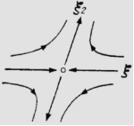 |
| Unstable node |
Im(λ1), Im(λ2), …, Im(λn) = 0 and Re(λ1), Re(λ2), …, Re(λn) > 0 Implemented by eode_is_unsnod() |
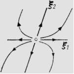 |
| Stable focus |
Im(λ1), Im(λ2), …, Im(λn) ≠ 0 and Re(λ1), Re(λ2), …, Re(λn) < 0 Implemented by eode_is_stafoc() |
 |
| Center |
Im(λ1), Im(λ2), …, Im(λn) ≠ 0 and Re(λ1), Re(λ2), …, Re(λn) = 0 Implemented by eode_is_centre() |
 |
| Unstable focus |
Im(λ1), Im(λ2), …, Im(λn) ≠ 0 and Re(λ1), Re(λ2), …, Re(λn) > 0 Implemented by eode_is_unsfoc() |
 |
In the last section, we obtained an equilibrium point (0.3333, 0.3333). The outputs from the following code show that this point is a saddle.