eq1 <- function(x, y, r1 = 4, a11 = 1, a12 = 2) (r1 - a11 * x - a12 * y) * x
eq2 <- function(x, y, r2 = 1, a21 = 2, a22 = 1) (r2 - a21 * x - a22 * y) * y
x <- eode(dxdt = eq1, dydt = eq2)
x
## An ODE system: 2 equations
## equations:
##   dxdt = (r1 - a11 * x - a12 * y) * x
##   dydt = (r2 - a21 * x - a22 * y) * y
## variables: x y
## parameters: r1 = 4, a11 = 1, a12 = 2, r2 = 1, a21 = 2, a22 = 1
## constraints: x<1000 x>0 y<1000 y>02 ODE Expression in ‘ecode’
2.1 An ‘ecode’ Object
An ‘ecode’ object is a standard way to store information of an ODE system in package ‘ecode’. It is the most important data type in the package. To define an ODE system, users must first create an ‘ecode’ object. This can be done by the constructor function eode(),
Here we define a system that has two state variables x, y,
\[ dx/dt=(r_1-a_{11}x-a_{12}y)\cdot x \]
\[ dy/dt=(r_2-a_{21}x-a_{22}y)\cdot y \]
where parameter \(r_1=4,\ a_{11}=1,\ a_{12}=2,\ r_2=1,\ a_{21}=2,\ a_{22}=1\). The model is called Lotka–Volterra competition equations. It describes how two species compete with each other for higher survival. Variable x,y is the population size for two species. The population growth rate of the first species is given by \(r_1-a_{11}x-a_{12}y\), where \(r_1\) is called the intrinsic growth rate, the potential rate of growth without any competitors, \(a_{11}\) the linear reduction effect on population growth caused by intra-specific competition, and \(a_{12}\) the reduction effect caused by interspecific competition. The second equation can be analysed in the same way.
In ‘ecode’, all ODEs should be defined as an R function. Arguments without default values (such as x, y) are automatically processed as state variables, while arguments with default values are model parameters. The function body defines phase velocity vectors. When all equations are ready, the function eode() can be used to finalise an ODE object. Because there are two state variables x and y, we must specify the named arguments dxdt and dydt in the function head. Argument dxdt should be the R function that defines the phase velocity vector of variable x, and argument dydt for phase velocity vector of variable y.
When sending a command x to the console, it will print information of the ODE system. It can be seen from the outputs that the system has two variables, six model parameters, and automatically generated constraints on variable ranges 0 < x, y < 1000.
2.2 System Setting
System boundary enables the phase point to move in a meaning range. The range 0 < x < 1000 is automatically generated by the function eode(). This means that every time when the phase point falls outside this range, a simulation will be stopped. Users can modify the valid range of system variables using the argument constraint,
x <- eode(dxdt = eq1, dydt = eq2, constraint = c("x<100", "x>20", "y<20"))
x
## An ODE system: 2 equations
## equations:
##   dxdt = (r1 - a11 * x - a12 * y) * x
##   dydt = (r2 - a21 * x - a22 * y) * y
## variables: x y
## parameters: r1 = 4, a11 = 1, a12 = 2, r2 = 1, a21 = 2, a22 = 1
## constraints: x<100 x>20 y<20 y>0
The argument constraint accepts an R vector that specifies new boundary conditions to overwrite the old ones. Boundaries that are not overwritten will remain at (0, 1000). The function eode_set_constraint can also be used to change the boundary condition of an existing ODE system.
eq1 <- function(x, y, r1 = 4, a11 = 1, a12 = 2) (r1 - a11 * x - a12 * y) * x
eq2 <- function(x, y, r2 = 1, a21 = 2, a22 = 1) (r2 - a21 * x - a22 * y) * y
x <- eode(dxdt = eq1, dydt = eq2, constraint = c("x<100", "x>20", "y<20"))
x_new <- eode_set_constraint(x, new_constraint = c("x<100", "x>20", "y<20"))
x_new
## An ODE system: 2 equations
## equations:
##   dxdt = (r1 - a11 * x - a12 * y) * x
##   dydt = (r2 - a21 * x - a22 * y) * y
## variables: x y
## parameters: r1 = 4, a11 = 1, a12 = 2, r2 = 1, a21 = 2, a22 = 1
## constraints: x<100 x>20 y<20 y>0
Model parameters can also be changed after an ‘ecode’ object is created. This is achieved by the function eode_set_parameter,
eq1 <- function(x, y, r1 = 4, a11 = 1, a12 = 2) (r1 - a11 * x - a12 * y) * x
eq2 <- function(x, y, r2 = 1, a21 = 2, a22 = 1) (r2 - a21 * x - a22 * y) * y
x <- eode(dxdt = eq1, dydt = eq2, constraint = c("x<100", "x>20", "y<20"))
x_new <- eode_set_parameter(x, ParaList = list(r1 = 6, a21 = 4))
x_new
## An ODE system: 2 equations
## equations:
##   dxdt = (r1 - a11 * x - a12 * y) * x
##   dydt = (r2 - a21 * x - a22 * y) * y
## variables: x y
## parameters: r1 = 6, a11 = 1, a12 = 2, r2 = 1, a21 = 4, a22 = 1
## constraints: x<100 x>20 y<20 y>0
Phase Velocity Vector Field
By exploring the phase velocity vector field, one gets a rough idea where phase points move quickly and where equilibria might exist. This is done by simply calling the function plot(),
eq1 <- function(x, y, r1 = 4, a11 = 1, a12 = 2) (r1 - a11 * x - a12 * y) * x
eq2 <- function(x, y, r2 = 1, a21 = 2, a22 = 1) (r2 - a21 * x - a22 * y) * y
x <- eode(dxdt = eq1, dydt = eq2, constraint = c("x<2", "y<2"))
plot(x)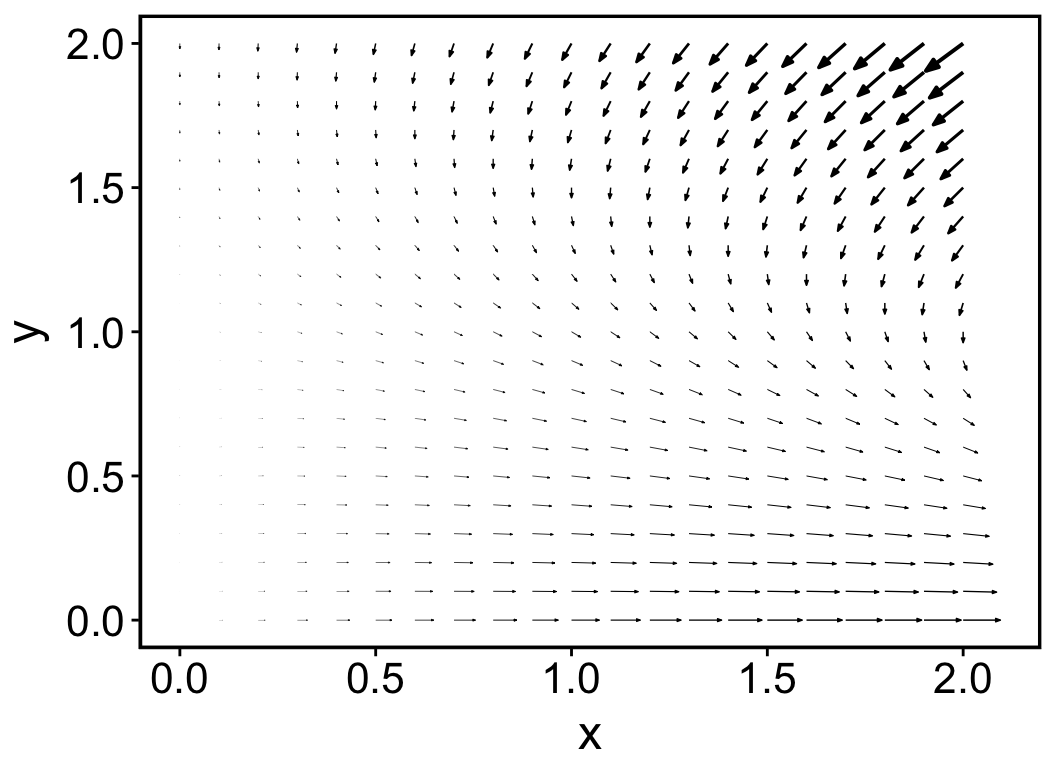
The result is shown in Figure 2.1. Since all arrows point to the negative y axis until y = 0, we can infer that species x outcompete species y even when x has a very small population size initially.
For ODE systems of more than two variables, it is difficult to visualise the phase velocity vector field. In this case, a two-dimensional subspace of the phase plane will be plotted. This means that only two variables will be shown in the vector field, and the remaining variables will be fixed. For example, a system with four state variables x1, x2, x3, x4 (0 < x1, x2, x3, x4 < 10) has a four-dimensional phase plane. The plot() function will by default sketch a subspace spanned by x1, x2, while the remaining variables will be automatically set as 5, the middle value of the valid range. It is up to the user to decide which two variables to show up. Using the argument set_covar = list(x1 = 7, x2 = 5) for the function plot(), we can fix the variables x1, x2, and force variables x3, x4 to show up in the subspace.