Chapter 2 Sample collection and map
Many articles need to use maps to display some data. Professional drawing software such as ARCGIS is more expensive and takes a long time to learn. The advantage of drawing with R is that everyone can install R and R maps have no copyright issues and are easy to use. The main R packages used are ggplot2, sf, rnaturalearth, rnaturalearthdata, etc. When you need to modify the picture, you only need to modify the code, which eliminates the cumbersome modification of the picture.
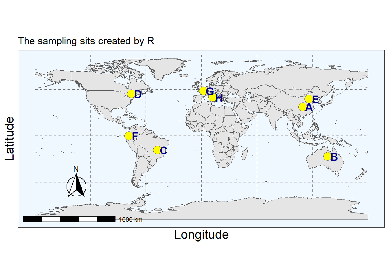
To determine the origin of the sample, so samples from different countries are collected, and the location of the origin needs to be marked on the map.
library(rnaturalearth)
library(rnaturalearthdata)
library(ggspatial)
library(sf)
library(ggplot2)
library(gpclib)
library(maptools)
library(maps)
library(mapdata)
library(sp)
library(raster)
library(RColorBrewer)
library(rgeos)
The sampling sits could be created by R:
setwd("C:/local_R/R-Cookbook-in-Food-Science/Dataset")
XY <- read.csv('XY.csv')##Coordinate data
##world map
world <- ne_countries(scale = "medium", returnclass = "sf")

theme_set(theme_bw())

##start with ggplot
g1 <- ggplot(data = world)+
  geom_sf() +
  geom_point(data=XY,aes(x=X,y=Y),pch=21,fill="yellow",col="grey40",size=5)+
  ##name positions
  geom_text(data= XY,aes(x=Code_X, y=Y, label=Code),
       color = "darkblue", fontface = "bold",size=5, check_overlap = FALSE)+
  labs(title="The sampling sits created by R")+
  xlab("Longitude") + ylab("Latitude")+
  ##set font size
  theme(axis.text=element_text(size=12),
        axis.title=element_text(size=16))+
 ##Insert compass and scale
  annotation_scale(location = "bl", width_hint = 0.5) +
  annotation_north_arrow(
  location = "bl", which_north = "true",
  pad_x = unit(0.75, "in"), pad_y = unit(0.5, "in"),
  style = north_arrow_fancy_orienteering)+
  theme(panel.grid.major = element_line(color = gray(.5),
  linetype = "dashed", size = 0.5),
  panel.background = element_rect(fill = "aliceblue"))

g1