Chapter 7 Principal component analysis
From this section, the machine learning will be discussed by foods data, the data from Mid-infrared spectroscopy will be used for Geographical origin of Extra Virgin Olive Oils (Quadram open dataset,2003).
First we use R for data clean and wrangling. Python will also be used for PCA plots.
7.2 Data wrangling
The raw data form are not suitable for R programming, therefore we need to transpose it ti suitable form.
## data transpose
oil_transpose <- as.data.frame(t(oil))

print(oil_transpose[1:10,1:5])
## V1 V2 V3 V4 V5
## V1 Sample Number: Group Code: Wavenumbers 798.892 800.8215
## V2 1 1 Greece 0.127523009 0.127949615
## V3 1 1 Greece 0.126498181 0.127130974
## V4 2 1 Greece 0.130411785 0.130675401
## V5 2 1 Greece 0.130022227 0.130406662
## V6 3 1 Greece 0.128601989 0.128789565
## V7 3 1 Greece 0.128217254 0.128282253
## V8 4 1 Greece 0.126174933 0.126732773
## V9 4 1 Greece 0.126466053 0.126915413
## V10 5 1 Greece 0.127060105 0.127551128## rename some col names to make data analysis easier
colnames(oil_transpose)=oil_transpose[1,]
oil_transpose <- oil_transpose[-1,]
library(dplyr)
oil_transpose <- rename(oil_transpose,c("Group" ="Group Code:",
"Number" ="Sample Number:",
"Countries" ="Wavenumbers"))
## Get transposed dataset
oil.data <- oil_transpose
print(oil.data[1:10,1:5])## Number Group Countries 798.892 800.8215
## V2 1 1 Greece 0.127523009 0.127949615
## V3 1 1 Greece 0.126498181 0.127130974
## V4 2 1 Greece 0.130411785 0.130675401
## V5 2 1 Greece 0.130022227 0.130406662
## V6 3 1 Greece 0.128601989 0.128789565
## V7 3 1 Greece 0.128217254 0.128282253
## V8 4 1 Greece 0.126174933 0.126732773
## V9 4 1 Greece 0.126466053 0.126915413
## V10 5 1 Greece 0.127060105 0.127551128
## V11 5 1 Greece 0.126812707 0.1274607437.3 Principal Component Analysis using R
The PCA is used to reduce the dimensionality of the spectral value, and initially explore the distribution of the sample.
The original data and related transformated data (MSC, SNV and Savitzky-Golay filtering) are used to obtain the PCA plots.
library(missMDA)
library(factoextra)
library(FactoMineR)
library(ggrepel)
library(ggplot2)
library(mixOmics)
library(EMSC)
library(pls)
library(prospectr)
7.3.1 Raw data PCA
Have a look at spectral of different pre-processing for MIR.
colors = c("#CD0000", "#EE7600", "#FFFF00", "#008B45")
col <- as.factor(oil.data$Countries)
group <- c("Greece","Italy","Portuga", "Spain")
RAW spectral
raw_spc <- oil.data[,4:573]

x <- as.numeric(colnames(raw_spc))
y <- t(raw_spc[ , ])

par(mar=(c(5,7,4,2)))

matplot(x, y,col = colors,
        type = 'l', lty = 1,
        xlab = 'Wavelength (nm)', ylab = 'Absorbance',main = "Raw",
        font.lab = 1,
        cex.main = 1, cex.axis = 1, cex.lab=2)
legend("topleft",
       title = "Country",
       xpd = F,ncol = 1,
       legend = group,
       col = col,
       fill = colors,
       bty = "n",
       cex = 1.5,
       text.col = "black", text.font = 1,
       horiz = F)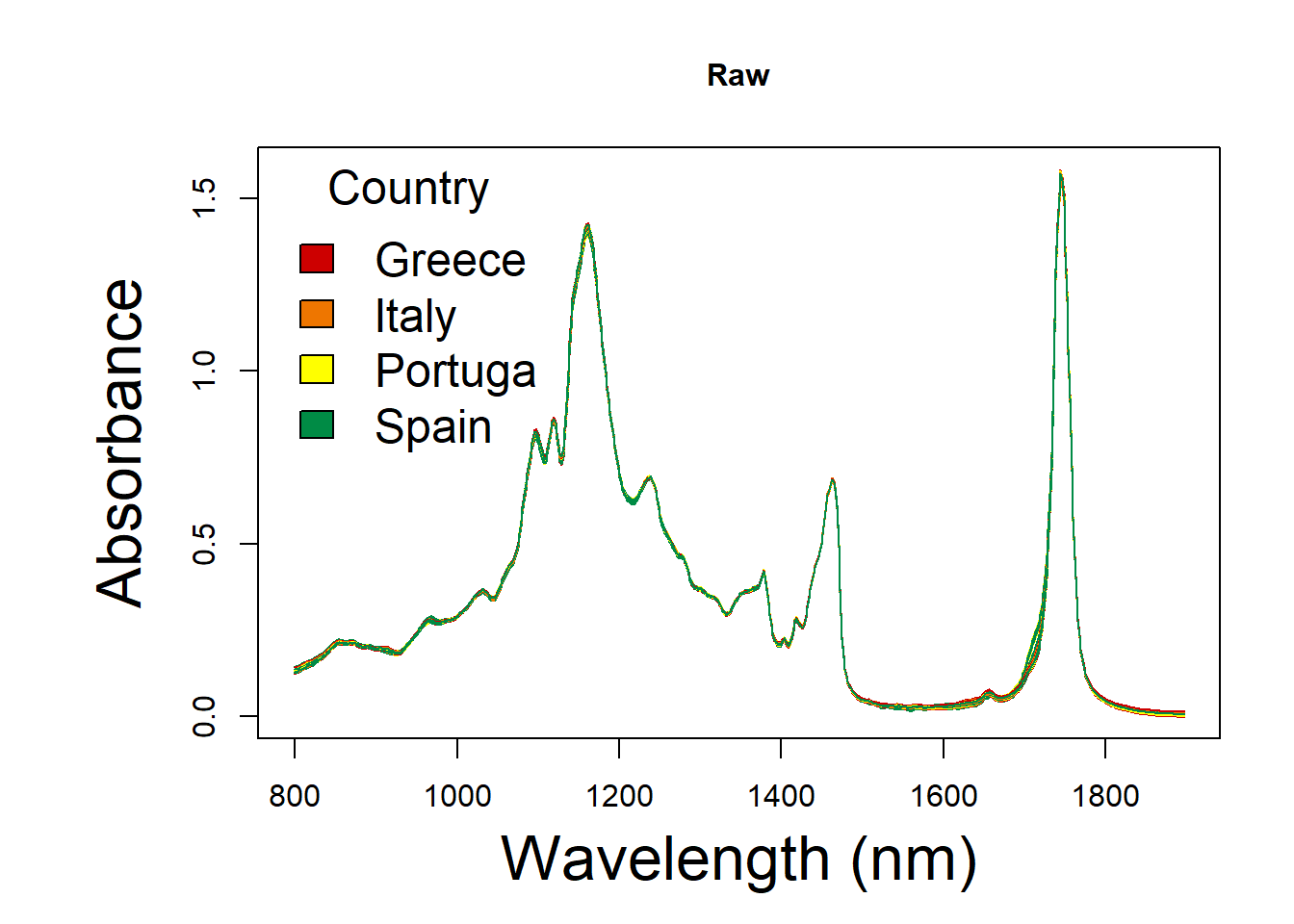
p1 <- recordPlot()df_raw <- oil.data[,4:573]
df <- as.data.frame(apply(df_raw, 2, as.numeric))
print(df[1:10,1:5])## 798.892 800.8215 802.751 804.6805 806.61
## 1 0.1275230 0.1279496 0.1292822 0.1311742 0.1335903
## 2 0.1264982 0.1271310 0.1285108 0.1303399 0.1325272
## 3 0.1304118 0.1306754 0.1320166 0.1338241 0.1360953
## 4 0.1300222 0.1304067 0.1320180 0.1340073 0.1362706
## 5 0.1286020 0.1287896 0.1300223 0.1320119 0.1344266
## 6 0.1282173 0.1282823 0.1296366 0.1317986 0.1340615
## 7 0.1261749 0.1267328 0.1282438 0.1298927 0.1317546
## 8 0.1264661 0.1269154 0.1282541 0.1299583 0.1320672
## 9 0.1270601 0.1275511 0.1289000 0.1306090 0.1329558
## 10 0.1268127 0.1274607 0.1287653 0.1306390 0.1331313oil.pca <- PCA(df,scale.unit = TRUE,ncp = 5,graph = TRUE)The PCA plot of raw Spectral
g1 <- fviz_pca_ind(oil.pca, geom.ind = "point",
                      col.ind = oil.data$Countries, # color by groups
                      palette = 'jco',
                      addEllipses = TRUE, ellipse.type = "convex",
                      legend.title = "Groups")+
  ggtitle("Oil - geographical-Raw Data")

g1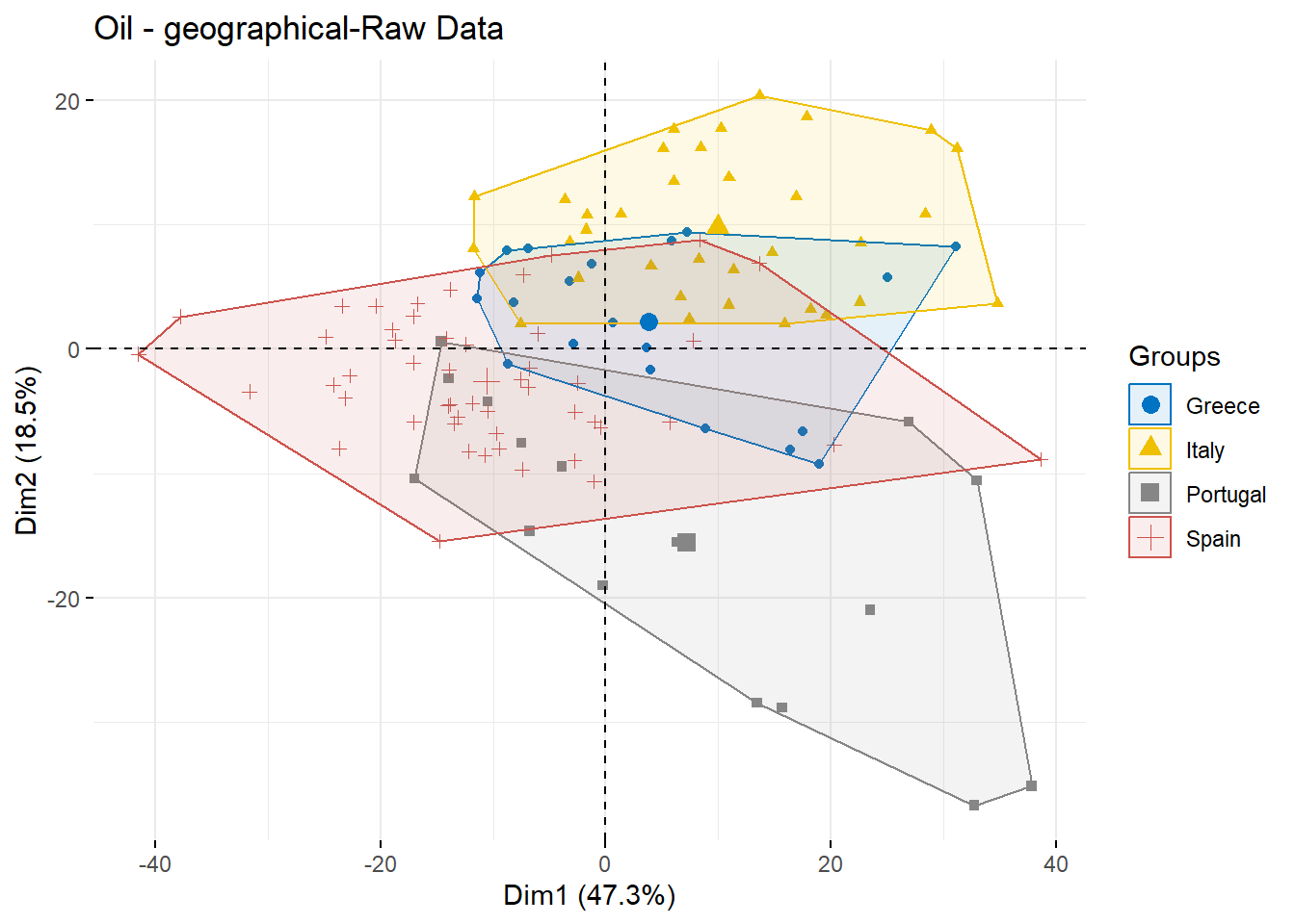
7.3.2 Standard Normal Variate
df_snv <- standardNormalVariate(df)

oil.snv <- cbind(oil.data[,1:3], df)
SNV spectral
x <- as.numeric(colnames(oil.snv))
y <- t(oil.snv[ , ])

par(mar=(c(5,7,4,2)))

matplot(x, y,col = colors, ylim = c(0,2),
        type = 'l', lty = 1,
        xlab = 'Wavelength (nm)', ylab = 'Absorbance',main = "SNV",
        font.lab = 1,
        cex.main = 1, cex.axis = 1, cex.lab=2)
legend("topleft",
       title = "Country",
       xpd = F,ncol = 1,
       legend = group,
       col = col,
       fill = colors,
       bty = "n",
       cex = 1.5,
       text.col = "black", text.font = 1,
       horiz = F)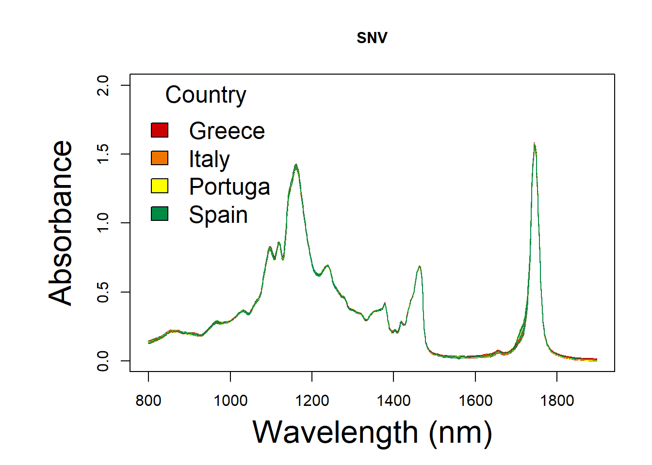
p3 <- recordPlot()The PCA plot of SNV Spectral
oil.snv.pca <- PCA(oil.snv[,4:563],scale.unit = TRUE,ncp = 5,graph = TRUE)g3 <- fviz_pca_ind(oil.snv.pca, geom.ind = "point",
col.ind = oil.snv$Countries, # color by groups
palette = 'jco',
addEllipses = TRUE, ellipse.type = "convex",
legend.title = "Groups")+
ggtitle("Oil - geographical-SNV")g3
7.3.3 Savitzky-Golay filtering
df_sg <- savitzkyGolay(
  X = df_snv,
  m = 1,
  p = 3,
  w = 11,
  delta.wav = 2
)

oil.sg <- cbind(oil.data[,1:3], df_sg)
Savitzky-Golay spectral
x <- as.numeric(colnames(oil.sg))
y <- t(oil.sg[ , ])

par(mar=(c(5,7,4,2)))

matplot(x, y,col = colors, ylim = c(-0.3,0.3),
        type = 'l', lty = 1,
        xlab = 'Wavelength (nm)', ylab = 'Absorbance',main = "Savitzky-Golay",
        font.lab = 1,
        cex.main = 1, cex.axis = 1, cex.lab=2)
legend("topleft",
       title = "Country",
       xpd = F,ncol = 2,
       legend = group,
       col = col,
       fill = colors,
       bty = "n",
       cex = 1.5,
       text.col = "black", text.font = 1,
       horiz = F)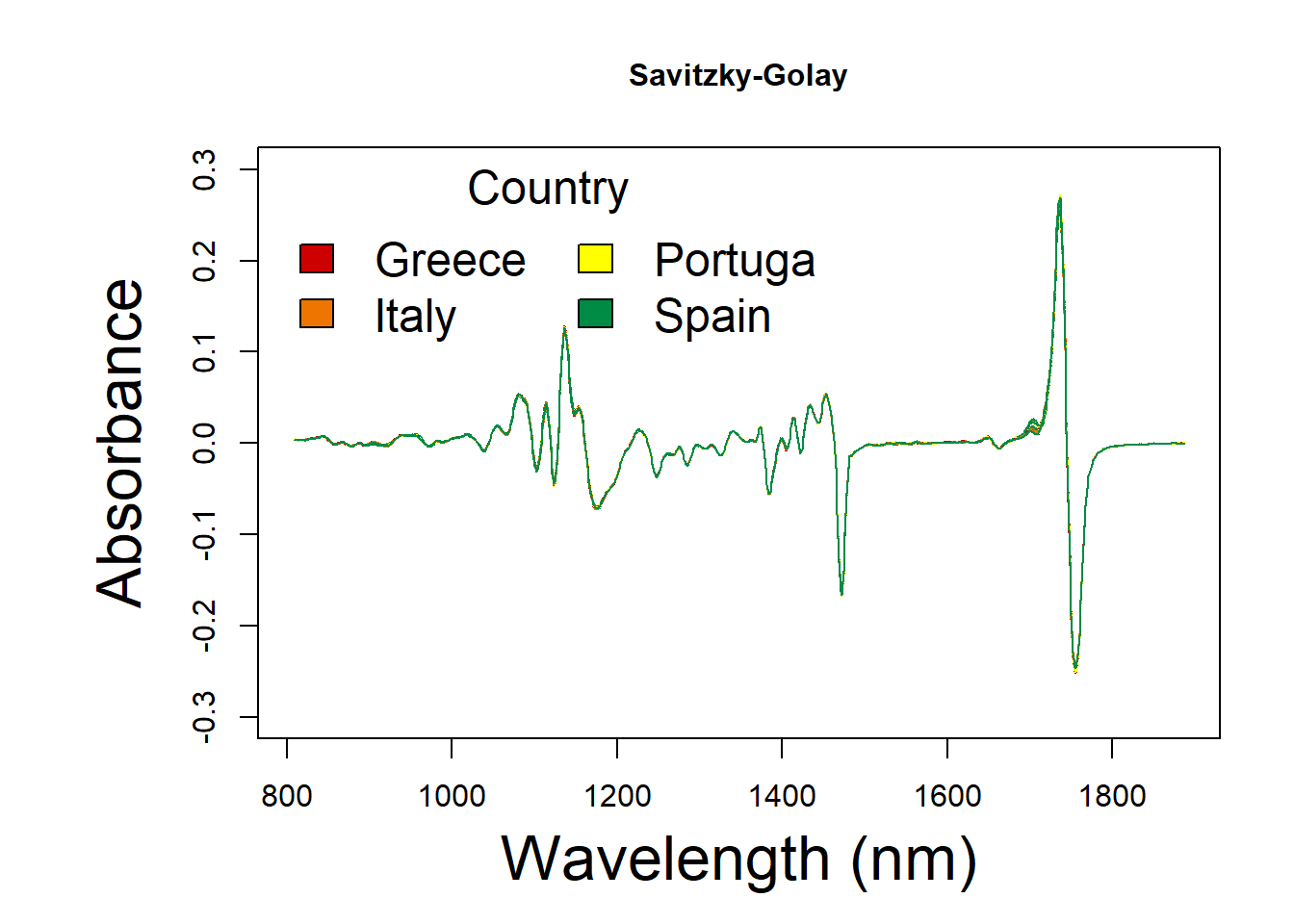
p4 <- recordPlot()p4
The PCA plot of Savitzky-Golay Spectral:
oil.sg.pca <- PCA(oil.sg[,4:563],scale.unit = TRUE,ncp = 5,graph = TRUE)g4 <- fviz_pca_ind(oil.sg.pca, geom.ind = "point",
col.ind = oil.sg$Countries, # color by groups
palette = 'jco',
addEllipses = TRUE, ellipse.type = "convex",
legend.title = "Groups")+
ggtitle("Oil - geographica-SG")g4
7.3.4 PCA plots comparations
library(cowplot)
library(ggpubr)
ggarrange(g1,g3,g4,
          labels = c("A", "B", "C"),
          ncol = 2, nrow = 2)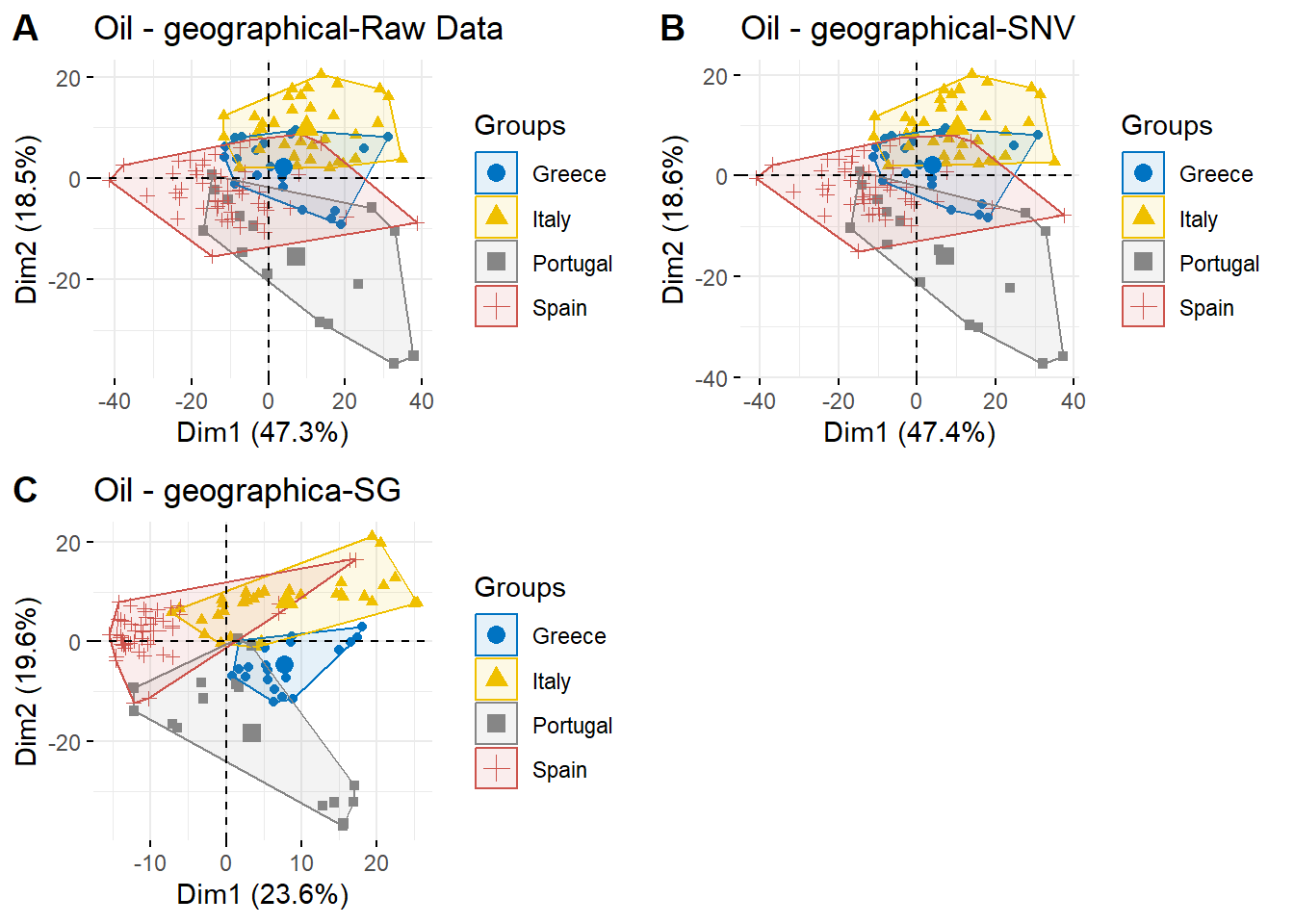
According to PCA plots, the best option is use RAW-SNV data set, therefore only RAW-snv transformated data will be used in the following data analysis such as classification models.