Assignment 3 Two Sample Test
3.1 Paired vs Unpaired t-test
Paired t-test is used to evaluate differences between two sets of results taken from the same sample. Since the values are dependent, taking their difference (Ex: diff = after - before) essentially transforms the paired t-test into a one-sample t-test, with \(H_0: \text{diff} =\bar{x}_1 - \bar{x}_0 = 0\) and \(\text{df} = n-1\).
Unpaired t-test is also refered as two sample t-test. In this case your samples are independent, with \(\text{df} = n_1 + n_2 - 2\) assuming equal/pooled variances between your two samples. However if we assumed unequal variance (which R does by default), you perform a Welch’s t-test (also known as unequal variances/unpooled t-test). The degrees of freedom formula for Welch’s t-test is more complicated.
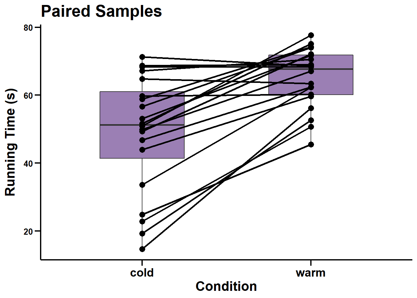
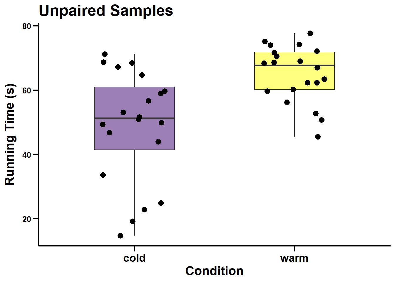
I will use the rats running time under hot vs cold conditions dataset (n = 20) to conduct both a paired and two-sample t-test. Of course, do not use 2-sample t-test when you have paired data and vice versa. For my two-sample t-test I will assume they are unpaired (n = 40).
dataset3 <- fread("C:/Users/Elspectra/Desktop/Core Course TA/Week 3/running_times.csv")

#Paired t-test.
result3_paired <- t.test(x = dataset3[["warm"]],
                         y = dataset3[["cold"]],
                         alternative = "two.sided",
                         paired = TRUE)
#Unpaired t-test. Keep in mind we are assuming two samples of n=20 rats in this case. Do not perform 2-sample t-test for a paired sample.
result3_unpaired <- t.test(x = dataset3[["warm"]],
                           y = dataset3[["cold"]],
                           alternative = "two.sided")

#Building the table this way is pretty unimpressive. Wonder if there is a way to loop it. The issue I encountered was that the variable name must be explicitly stated, which cant be done in a loop.
result3_summary = data.table(Test = c(result3_paired[["method"]], result3_unpaired[["method"]]),
                             Method = c(result3_paired[["alternative"]], result3_unpaired[["alternative"]]),
                             t_statistic = c(round(result3_paired[["statistic"]], 2), round(result3_unpaired[["statistic"]], 2)),
                             df = c(round(result3_paired[["parameter"]], 1), round(result3_unpaired[["parameter"]], 1)),
                             p_value = c(round(result3_paired[["p.value"]], 5), round(result3_unpaired[["p.value"]], 5)))

#datatable() does not seem to work in bookdown. Therefore will use knitr as alternative to display tables.
knitr::kable(result3_summary)| Test | Method | t_statistic | df | p_value |
|---|---|---|---|---|
| Paired t-test | two.sided | 5.73 | 19.0 | 0.00002 |
| Welch Two Sample t-test | two.sided | 3.73 | 28.2 | 0.00085 |
I have listed these two tests side by side to show differences in how they can be visually reported.
Note: once again, these results should be interpreted independently and not side by side. A paired t-test should never be used for independent samples, for example.
#To generate a multi-category scatter plot, we first have to modify the dataset and add a 'condition' variable.
dataset3 <- cbind(ID = rownames(dataset3), dataset3)

dataset3_edit <- data.table(ID = character(0),
                            condition = character(0),
                            time = numeric(0))

#This loop allows me to stack one condition and its values on top of the other.
for(i in 2:(length(names(dataset3)) - 1)){
  dataset3_temp <- data.table(ID = dataset3[["ID"]],
                              condition = names(dataset3)[i],
                              time = dataset3[[i]])
  dataset3_edit = bind_rows(dataset3_edit, dataset3_temp)
}

ggscatter_paired <- ggplot(data = dataset3_edit, aes(x = condition, y = time)) +
                    geom_boxplot(fill = "#38006A", width = 0.5, alpha = 0.5) +
                    geom_point(shape = 21, size = 3, fill = "black") +
                    geom_line(aes(group = ID), size = 1) +
                    labs(title = "Paired Samples", x = "Condition", y = "Running Time (s)") +
                    theme(panel.background = element_blank(),
                          axis.line = element_line(size = 0.75, color = "black"), #make main x,y axis line black
                          axis.ticks = element_line(size = 0.75, color = "black"),
                          axis.ticks.length.y = unit(.25, "cm"), #how long the axis ticks are
                          axis.ticks.length.x = unit(.25, "cm"),
                          axis.text.y = element_text(color = "black", face = "bold", size = 10),
                          axis.text.x = element_text(color = "black", face = "bold", size = 14),
                          axis.title = element_text(color = "black", face = "bold", size = 16),
                          axis.title.y = element_text(margin = margin(t=0,r=8,b=0, l=0)),
                          plot.title = element_text(color = "black", face = "bold", size = 20))

ggscatter_unpaired <- ggplot(data = dataset3_edit, aes(x = condition, y = time)) +
                      geom_boxplot(fill = c("#38006A", "yellow"), width = 0.5, alpha = 0.5) +
                      geom_point(position = position_jitter(width = 0.2), size = 3) +
                      labs(title = "Unpaired Samples", x = "Condition", y = "Running Time (s)") +
                      theme(panel.background = element_blank(),
                          axis.line = element_line(size = 0.75, color = "black"), #make main x,y axis line black
                          axis.ticks = element_line(size = 0.75, color = "black"),
                          axis.ticks.length.y = unit(.25, "cm"), #how long the axis ticks are
                          axis.ticks.length.x = unit(.25, "cm"),
                          axis.text = element_text(color = "black", face = "bold", size = 10),
                          axis.text.x = element_text(color = "black", face = "bold", size = 14),
                          axis.title = element_text(color = "black", face = "bold", size = 16),
                          axis.title.y = element_text(margin = margin(t=0,r=8,b=0, l=0)),
                          plot.title = element_text(color = "black", face = "bold", size = 20))

ggscatter_paired
ggscatter_unpaired

3.2 MGFs and their properties
What are moment generating functions
Moment generating functions (MGFs) represent an alternate way to specify the probability distribution of random variables.
Each distribution has their own unique MGF, given that it exists. \(E(e^{tx})\) can be derived by simplifying:
\(\begin{align} & \int_{-\infty}^{\infty}e^{tx}f_X(x)dx && \text{if X is continuous (pdf is known)} \\ & \sum_{x}e^{tx}P(X=x) && \text{if X is discrete (pmf is known)} \\ \end{align}\)
Note that the subscript ‘\(x\)’ in \(f_X\) or \(M_X\) is simply used denote the variable we are looking at. If we wanted to look at the MGF of a standard normal function of \(X\) for example, we would label it as \(M_{(x-\mu)/\sigma}(t)\).
Below is a table for some of the common distributions and their moment generating functions.
#Using latex in R code block apparently requires double slash: \\ instead of just one.
mgf_tbl <- data.table(Distribution = c("Binomial: $B(n,p)$", "Poisson: $Pois(\\lambda)$", "Normal: $N(\\mu,\\sigma^2)$"),
                   MGF = c("$(1-p+pe^t)^n$", "$e^{\\lambda(e^{t}-1)}$", "$e^{t\\mu + \\frac{1}{2}\\sigma^2t^2}$"),
                   "$\\frac{d}{dt}M_X(0)$" = c("$np$", "$\\lambda$", "$\\mu$"),
                   "$\\frac{d^2}{dt^2}M_X(0)$" = c("$n(n-1)p^2+np$", "$\\lambda+\\lambda^2$", "$\\sigma^2+\\mu^2$"))
knitr::kable(mgf_tbl)| Distribution | MGF | \(\frac{d}{dt}M_X(0)\) | \(\frac{d^2}{dt^2}M_X(0)\) |
|---|---|---|---|
| Binomial: \(B(n,p)\) | \((1-p+pe^t)^n\) | \(np\) | \(n(n-1)p^2+np\) |
| Poisson: \(Pois(\lambda)\) | \(e^{\lambda(e^{t}-1)}\) | \(\lambda\) | \(\lambda+\lambda^2\) |
| Normal: \(N(\mu,\sigma^2)\) | \(e^{t\mu + \frac{1}{2}\sigma^2t^2}\) | \(\mu\) | \(\sigma^2+\mu^2\) |
Moments of a MGF
A given distribution’s moment generating function can be used to calculate moments: \(E(X^{n})\), where \(n\) represents the moment (n=1: first moment, n=2, second moment, etc…).
This means that for random variable \(X\), the first derivative of its MGF evaluated at \(t=0\) represents \(E(X)\), aka the mean of \(X\).
The second derivative of the MGF evaluated at \(t=0\) represents \(E(X^2)\). We then arrive at the variance of \(X\) with a bit of computation:
\(Var(X) = E(X-E(X))^2 = E(X^2) - E(X)^2 = M^{''}_X(0) - (M^{'}_X(0))^2\)
Note: The MGF is just one of many ways to calculate the mean and variance of a distribution. It can also be used to characterize an infinite number of moments, but not vice versa.
Characterizing a distribution using MGFs
A major usefulness of MGFs is their ability to determine the distribution of a random variable.
We will be using this property of moment generating functions to prove the central limit theorem: how sample means \(\bar{X}\) from any distribution converges to normality as sample size \(n \to \infty\).
Note: I hear the proof of the above theorem is complicated and uses the uniqueness property of laplace transforms. Probably not that useful to know.
MGF of functions of random variables
When the MGF for a random variable exists, it is easy to find the MGF of functions of a random variable using the following theorem:
\(\begin{align} M_X(t) & = E(e^{tX}) \\[4pt] M_{aX+b}(t) & = E(e^{t(aX+b)}) \\[4pt] & = E(e^{taX}e^{tb}) \\[4pt] & = e^{tb}E(e^{(ta)X}) && \text{Expectation of a constant is the constant} \\[4pt] & = e^{tb}M_X(ta) \\ \end{align}\)
The proof is strait forward and follows similar logic as in theorem 3.2.
3.3 Taylor series approximation
Taylor series can help us approximate a function at some desired point (usually 0) into a polynomial.
Definition 3.3 If a function \(g(x)\) has derivatives of order \(r\), that is, if \(g^{(r)}(x) = \frac{d^r}{dx^r}g(x)\) exists (indefinitely differentiable), then the taylor polynomial of order \(r\) at some desired point \(a\) is: \(\begin{align} T_r(x) & = \sum_{i=0}^{r}\frac{g^{(i)}(a)}{i!}(x-a)^i && \text{general form} \\ & = g(a) + \frac{g^`(a)}{1!}(x-a) + \frac{g^{``}(a)}{2!}(x-a)^2 + \frac{g^{```}(a)}{3!}(x-a)^3 + ... && \text{expanded form} \\[8pt] T_r(x) & = g(0) + \frac{g^`(0)}{1!}x + \frac{g^{``}(0)}{2!}x^2 + \frac{g^{```}(0)}{3!}x^3 + ... && \text{g(x) evaluated at 0} \\ \end{align}\)
where \(T_r(x)\) represents the taylor approximation polynomial of function \(g(x)\).
For the statistical application of taylor’s theorem, we are most concerned with the first-order taylor series, that is, an approximation using just the first derivative: \(g(a) + g^`(a)(x-a) + \text{Remainder}\).
3.4 More on Central Limit Theorem
Now we are ready to demonstrate the central limit theorem (theorem, followed by proof).
Let \(G_n(x)\) denote the cumulative density function (cdf) of \(\sqrt{n}(\bar{X}_n - \mu)/\sigma\). Then for any \(-\infty \lt x \lt \infty\), \[\lim\limits_{n \to \infty}G_n(x) = \int_{-\infty}^{x}\frac{1}{2\pi}e^{-y^{2}/2}dy\]
This theorem essentially states that as sample size increases, the function \(\sqrt{n}(\bar{X}_n - \mu)/\sigma\) approaches a standard dormal distribution \(N(0,1)\).
Recall how we standardized the sample means \(\bar{X}\) (of any size) for a normally distributed variable \(X \sim N(\mu, \sigma)\) in chapter 2.8:
\[\frac{\bar{X} - \mu}{\sigma/\sqrt{n}} \sim N(0,1)\]
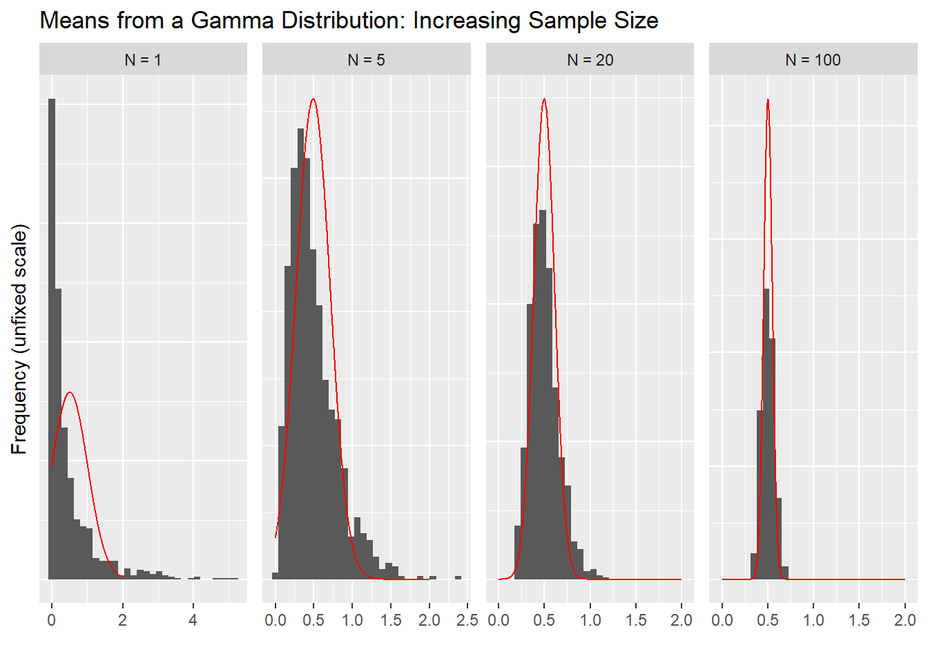
The central limit theorem tells us that resulting means \(\bar{X}\) of samples coming from any distribution becomes approximately normal as the sample size increases. We can prove the central limit theorem by showing that the MGF of means \(\bar{X}\) coming from any distribution equals the MGF of a normal distribution as sample size approaches \(\infty\).
Note: the CLT approximates the distribution of the sample mean \(\bar{X}\), not the distribution of the random variable itself \(X\).
Proof. Let \(Y_i = (X_i - \mu)/\sigma\) be the standardized random variable (coming from any distribution), and let \(M_Y(t)\) denote the common MGF of the \(Y_i\)s. Since
\(\begin{align} \frac{\sqrt{n}(\bar{X}_n - \mu)}{\sigma} = \sqrt{n}(\frac{1}{n}\sum_{i=1}^{n}\frac{X_i - \mu}{\sigma}) = \sqrt{n}(\frac{1}{n} \sum_{i=1}^{n}Y_i) = \frac{1}{\sqrt{n}} \sum_{i=1}^{n}Y_i \end{align}\)
we have, from the properties of MGFs,
\(\begin{align} M_{\sqrt{n}(\bar{X}_n - \mu)/\sigma}(t) & = M_{\sum_{i=1}^{n}Y_{i}/\sqrt{n}}(t) \\ & = M_{\sum_{i=1}^{n}Y_{i}}(\frac{t}{\sqrt{n}}) && \text{Theorem 3.2} \\ & = (M_Y(\frac{t}{\sqrt{n}}))^n && \text{Theorem 3.3, $Y_i$s independent & identially distributed} \\ \end{align}\)
We use taylor expansion to approximate \(M_Y(\frac{t}{\sqrt{n}})\) around 0:
\(\begin{align} M_Y(\frac{t}{\sqrt{n}}) & = M_Y(0) + \frac{M^{`}_Y(0)}{1!}(t/\sqrt{n}) + \frac{M^{``}_Y(0)}{2!}(t/\sqrt{n})^2 + R_Y(\frac{t}{\sqrt{n}}) \\ & = 1 + \frac{(t/\sqrt{n})^2}{2} + R_Y(\frac{t}{\sqrt{n}}) \\ \end{align}\)
Since Y is standardized, we know that its first moment \(M^{`}_Y(0)\) is 0, and second moment \(M^{``}_Y(0)\) is 1. The zeroth moment \(M_Y(0)\) represents the total probability, which is 1.
\(R_Y(\frac{t}{\sqrt{n}})\) represents the collective remainder term for this taylor expansion.
Now to evaluate our original \((M_Y(\frac{t}{\sqrt{n}}))^n\) as sample size \(n \to \infty\):
\(\begin{align} \lim\limits_{n \to \infty}(M_Y(\frac{t}{\sqrt{n}}))^n & = \lim\limits_{n \to \infty}(1 + \frac{(t/\sqrt{n})^2}{2} + R_Y(\frac{t}{\sqrt{n}})^n \\[5pt] & = \lim\limits_{n \to \infty}(1 + \frac{1}{n}(\frac{t^2}{2} + nR_Y(\frac{t}{\sqrt{n}})))^n \\[5pt] & = e^{t^2/2} && \text{see remarks 1 & 2} \\ \end{align}\)
Therefore, we have demonstrated that as sample size \(n \to \infty\), the MGF \(M_{\sqrt{n}(\bar{X}_n - \mu)/\sigma}(t)\) is equivalent to the MGF of a standard normal distribution (see remark 3).
Remark 1: what happens to the remainder
Taylor’s theorem states that the remainder of the approximation always tends to 0 faster than the highest-order non-remainder term.
Therefore, our remainder \(R_Y(\frac{t}{\sqrt{n}})\) will decay faster than our second order term \(\frac{(t/\sqrt{n})^2}{2}\) (the highest before our remainder):
\(\begin{align} & \lim\limits_{n \to \infty}\frac{R_Y(t/\sqrt{n})}{1/\sqrt(n)} = \lim\limits_{n \to \infty}nR_Y(\frac{t}{\sqrt{n}}) = 0 \\ \end{align}\)
Note that we removed constants which plays no role in the limit. In our ratio, our numerator decays faster than our denominator, Therefore the ratio approaches 0 as sample size \(n \to \infty\).
Remark 2: property of limitsBy setting \(a_n = \frac{t^2}{2} + nR_Y(\frac{t}{\sqrt{n}})\),
\(\begin{align} \lim\limits_{n \to \infty}(1 + \frac{1}{n}(\frac{t^2}{2} + nR_Y(\frac{t}{\sqrt{n}})))^n = \lim\limits_{n \to \infty}(1 + \frac{1}{n}(a))^n \\ \end{align}\)
Using remark 1 we can show that as sample size \(n \to \infty\): \(\begin{align} \lim\limits_{n \to \infty}(\frac{t^2}{2} + nR_Y(\frac{t}{\sqrt{n}})) = t^2/2 \\ \end{align}\)
Therefore: \(\begin{align} \lim\limits_{n \to \infty}(1 + \frac{1}{n}(a))^n = e^{t^2/2} \\ \end{align}\)
Remark 3: MGF of the standard normal distribution We can show that the MGF for \(N(0,1)\) is \(e^{t^2/2}\):
\(\begin{align} M_X(t) & = E(e^{tx}) && \text{definition of MGF} \\[6pt] & = \int_{-\infty}^{\infty}e^{tx}f(x)dx && \text{definition of expectation} \\[6pt] & = \int_{-\infty}^{\infty}e^{tx}\frac{1}{\sqrt{2\pi}}e^{(-\frac{1}{2}x^2)} && \text{pdf of standard normal distribution} \\[6pt] & = \int_{-\infty}^{\infty}\frac{1}{\sqrt{2\pi}}e^{(-\frac{1}{2}x^2 + tx)} && \text{notice we can complete the square} \\[6pt] & = \int_{-\infty}^{\infty}\frac{1}{\sqrt{2\pi}}e^{(-\frac{1}{2}(x^2 - 2tx + t^2) + \frac{1}{2}t^2)} && \text{multiple & divide by $\frac{1}{2}e^{t^2}$} \\[6pt] & = e^{t^2/2}\int_{-\infty}^{\infty}\frac{1}{\sqrt{2\pi}}e^{(-\frac{1}{2}(x - t)^2)} && \text{integral now represents cdf of $N(t, 1)$, which = 1} \\[6pt] & = e^{t^2/2} \\ \end{align}\)
3.5 Visualizing CLT Approximation
x = data.table(ID = 1,
               sample_size = 1,
               fact = "N = 1",
               dat = rgamma(1000, 0.5, 1))
x5 = data.table(ID = 2,
                sample_size = 5,
                fact = "N = 5",
                dat = replicate(1000, mean(rgamma(5, 0.5, 1))))
x20 = data.table(ID = 3,
                 sample_size = 20,
                 fact = "N = 20",
                 dat = replicate(1000, mean(rgamma(20, 0.5, 1))))
x100 = data.table(ID = 4,
                  sample_size = 100,
                  fact = "N = 100",
                  dat = replicate(1000, mean(rgamma(100, 0.5, 1))))
x_dat = bind_rows(x, x5, x20, x100)
x_dat$fact <- factor(x_dat$fact, levels = c("N = 1", "N = 5", "N = 20", "N = 100"))

norm_tbl <- data.table(predicted = numeric(0),
                       fact = character(0))

for(i in 1:4){
  a <- data.table(predicted = rnorm(1000, mean = 0.5, sd = 0.5/sqrt(x_dat$sample_size[x_dat$ID == i])),
                  fact = paste0("N = ", x_dat$sample_size[x_dat$ID == i]))
  norm_tbl <- bind_rows(norm_tbl, a)
}

norm_tbl$fact <- factor(norm_tbl$fact, levels = c("N = 1", "N = 5", "N = 20", "N = 100"))

grid <- with(norm_tbl, seq(0, 2, length = 1000))
normaldens <- ddply(norm_tbl, "fact", function(df) {
  data.table(predicted = grid,
             density = dnorm(grid, mean(df$predicted), sd(df$predicted)))
})

ggplot(data = x_dat) +
  geom_histogram(aes(x = x_dat$dat, y= ..density..), bins = 30) +
  geom_line(aes(x = normaldens$predicted, y = normaldens$density), colour = "red") +
  facet_wrap(~ fact, scales = "free", ncol = 4) +
  labs(title = "Means from a Gamma Distribution: Increasing Sample Size", x = "", y = "Frequency (unfixed scale)") +
  theme(axis.text.y = element_blank(),
        axis.ticks.y = element_blank())

#Need a method to prevent automatic scaling to the normal overlay (dependent on grid). I want to scale by my histogram.