Assignment 2 One Sample Test
2.1 Introduction
White blood cell (WBC) count, in #/ml blood, is my variable of interest. This is one of the primary clinical variables measured from patient blood, and is important for accessing patient immune condition.
2.2 Measurement
A list of 35 WBC results will be collected from Dr. Magnotti’s lab. These screening results come from healthy patients enrolled in a phase 1 safety trial.
2.3 Prediction
Since the WBC results were collected from healthy patients, I hypothesize that the mean WBC count will fall around 7500/ml blood. This number lies in between the normal WBC range of 4000-11000/ml, published by WebMD. To test my prediction, I plan to perform a 2-tailed t-test using the sample collected against H0: 7500/ml. An abnormal mean WBC count would suggest some underlying issue in the patients screened.
2.4 Results
dataset2 <- fread("C:/Users/Elspectra/Desktop/Core Course TA/Week 2/white_blood_cell_counts.csv")
result2 <- t.test(dataset2[["wbc"]],
                  mu = 7500,
                  alternative = "two.sided",
                  conf.level = 0.95)

# A 2-tailed one sample t-test showed that there was a statistically significant difference between the sample mean of `r round(result2$estimate)`/ml and my H~0~: 7500/ml,
# **t**(`r result2$parameter`) = `r round(result2$statistic, digits = 3)`, **p** = `r round(result2$p.value, digits = 3)`.
# The sample mean had a standard error of `r round(result2$stderr)`, and carried a 95% confidence interval between [`r round(result2$conf.int[1])`, `r round(result2$conf.int[2])`].
A 2-tailed one sample t-test showed that there was a statistically significant difference between the sample mean of 7792/ml and my H0: 7500/ml, t(34) = 2.295, p = 0.028. The sample mean had a standard error of 127, and carried a 95% confidence interval between [7533, 8050].
#Generally for ggplot elements, things which come later will layer in front of things coming before.
#This example only scratches the surface of what ggplot2 can do in terms of plot customization. Here we try to match the prism univariate scatter plot in R.
ggscatter <- ggplot(data = dataset2, aes(x = "", y = dataset2[["wbc"]], group = 1)) +
             geom_point(position = position_jitter(width = 0.2), size = 2) + #adding some jitter to the plotted dots. Prism does this automatically
             geom_errorbar(aes(ymin = mean(dataset2[["wbc"]]) - sd(dataset2[["wbc"]]), ymax = mean(dataset2[["wbc"]]) + sd(dataset2[["wbc"]])), width = 0.3, color = "red", size = 1) + #note that geom_errorbar will not plot the mean.
             geom_point(aes(y=mean(dataset2[["wbc"]])), size = 3, color = "red") + #add separate point to represent the mean
             annotate("text", x=Inf, y=Inf, label = paste0("N = ", nrow(dataset2)), vjust = 2, hjust = 1, fontface = "bold") + #fontface for bold syntax. vjust = vertical adjust, hjust = horizontal adjust. Here we annotate on top right.
             scale_y_continuous(limits = c(6000, 10000), expand = c(0,0)) + #define y-axis boundaries. Expand (0,0) sets furthest tick marks exactly on boundary.
             labs(title = "WBC Count in \nHealthy Patients", x = "WBC", y = "Count/ml Blood") +
             theme(panel.background = element_blank(), #make background white
                   axis.line = element_line(size = 0.75, color = "black"), #make main x,y axis line black
                   axis.ticks = element_line(size = 0.75, color = "black"),
                   axis.ticks.length.y = unit(.25, "cm"), #how long the axis ticks are
                   axis.ticks.length.x = unit(.25, "cm"),
                   axis.text = element_text(color = "black", face = "bold", size = 10),
                   axis.title = element_text(color = "black", face = "bold", size = 12),
                   axis.title.x = element_text(margin = margin(t=-8,r=0,b=0, l=0)), #top, right, bottom, left margins
                   plot.title = element_text(color = "black", hjust = 0))
ggscatter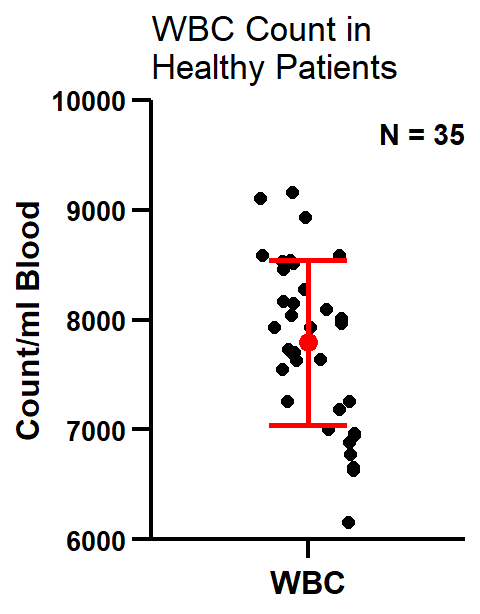
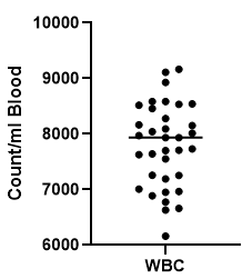
From the plot we can see that “jitter” in R does not reflect the distribution of our scatter. In order to mimick the “prism jitter effect” (shown below), we will need to install the ggbeeswarm package (not shown here).
2.5 Discussion
Upon performing a 2-tailed t-test, the sample mean for WBC count/ml blood in healthy patients (7792) was unexpectedly found to deviate from my expected mean (7500), p = 0.028. Therefore I reject my null hypothesis and conclude that the WBC count/ml mean is higher than the mid-point of the normal range provided by WebMD. On the other hand, my 95% CI for the mean fell well within the normal range. So while the distribution of WBC count in healthy patients is not centered around H0: 7500/ml, I can still conclude that the initial screening was performed on healthy patients.
2.6 Standard Deviation vs. Standard Error
When we typically speak of standard deviation, we are referring to the sample data \(X\):
\(\sigma_x = \sqrt{Var(X)} = \sqrt{\frac{\sum_{i=1}^{n}(X_i - \bar{X})^2}{n-1}}\).
On the other hand, standard error referrs to the ‘standard deviation’ of the sample mean \(\bar{X}\):
\(\sigma_{\bar{x}} = \sqrt{Var(\bar{X})} = \sqrt{Var(\frac{1}{n}\sum_{i=1}^{n}X_i)} = \sqrt{\frac{1}{n}Var(X_1)} = \sqrt{\frac{1}{n}\sigma^2_x} = \frac{\sigma_x}{\sqrt{n}}\).
Note: If random variable X is identitally distributed, then:
1. \(Var(X_1) = Var(X_i)\)
2. \(Var(\sum_{i=1}^{n}X_i) = nVar(X_1)\)
2.7 Population Variance vs. Sample Variance
Recall: variance is just standard deviation squared.
The population variance represents cases where the variance is derived from the population itself. The sample variance, as its name indicates, is the variance derived from a sample (subset) of your population.
When population variance is not known, the sample variance is used as an estimator to represent the population variance.
Sample variance is sometimes designated as \(S^2\) to distinguish itself from the population variance \(\sigma^2\).
However in statistics, whether or not the variance is known is often stated beforehand, and \(\sigma^2\) is used to represent either case. In section 2.6 above for example, \(\sigma_x\) represents sample standard dev. In this section and below, I will be using \(S\) to denote the sample standard dev.
The population standard deviation is derived through:
\(\sigma_x = \sqrt{\frac{\sum_{i=1}^{n}(X_i - \mu)^2}{n}}\), where \(\mu\) represents the population mean.
As shown in section 2.6, the sample standard deviation is derived through:
\(S_x = \sqrt{\frac{\sum_{i=1}^{n}(X_i - \bar{X})^2}{n-1}}\), where \(\bar{X}\) represents the sample mean.
Why divide \(n-1\) instead of \(n\) for the sample variance? Recall I mentioned that the sample variance was an estimate of the population variance. Logically, I would expect my sample variance to equal my population variance: \(E(S^2) = \sigma^2\).
Indeed by taking the expectation of the sample variance above, we obtain the population variance:
\(\begin{align*} E(S^2) & = E(\frac{1}{n-1}\sum_{i=1}^{n}(X_i - \bar{X})^2) \\ & = E(\frac{1}{n-1}(\sum_{i=1}^{n}X^2_i - n\bar{X}^2)) && \text{see remark 1}\\ & = \frac{1}{n-1}(nE(X^2_1) - nE(\bar{X}^2)) && \text{since X is identically distributed}\\ & = \frac{1}{n-1}(n(\sigma^2 + \mu^2) - n(\frac{\sigma^2}{n} + \mu^2)) && \text{see remark 2}\\ & = \frac{1}{n-1}((n-1)\sigma^2) = \sigma^2 \\ \end{align*}\)
By using \(\frac{1}{n-1}\), our sample variance \(S^2\) is an unbiased estimator of the population variance \(\sigma^2\). If we had used \(\frac{1}{n}\) instead, we would have acquired \(E(S^2) = \frac{n-1}{n}\sigma^2\). This bias is significant when sample size \(n\) is small (leading to under estimation of the true variance), and dissappears when sample size is large.
Remark 1:
\(\begin{align} \sum_{i=1}^{n}(X_i - \bar{X})^2 & = \sum_{i=1}^{n}(X^2_i - 2X_i\bar{X} + \bar{X}^2) \\ & = \sum_{i=1}^{n}X^2_i - 2\bar{X}\sum_{i=1}^{n}X_i + n\bar{X}^2 \\ & = \sum_{i=1}^{n}X^2_i - 2n\bar{X}^2 + n\bar{X}^2 \\ & = \sum_{i=1}^{n}X^2_i - n\bar{X}^2 \\ \end{align}\)
Remark 2:
Given \(X \sim N(\mu, \sigma^2)\):
- \(E(X^2)\) can be derived using the second moment of random variable \(X: M^{''}_X(0)\).
- \(E(\bar{X}^2)\) can be derived using the second moment of the random variable mean \(\bar{X}: M^{''}_\bar{X}(0)\).
More on moments and moment generating functions (MGFs) in chapter 3.2.
2.8 From z-test to t-test
Hypothesis testing is most often performed to determine whether the difference between your mean and some expected mean is significant. This depends on both the magnitude of the difference and the mean’s standard deviation (standard error). Note: formally, the function you are interested in testing is known as a statistic, and the value you are testing against is known as a parameter. The outcome, such as a z or t-value, is known as a test statistic.
What is the fundamental difference between a z-test and a t-test? For z-tests, the variance is known and comes from the population. For t-tests, the variance is estimated from a sample of the population. So why do z-values follow a standard normal distribution while t-values follow what is called a t-distribution? What is even a t-distribution? I feel the best way to address these questions is to work through the mathematical difference between a z-test and a t-test.
Let \(X_1,...,X_n\) be a random sample from a normal distribution \(N(\mu, \sigma^2)\), where variance \(\sigma^2\) is known.
The z-value is derived through:
\[\frac{\bar{X} - \mu}{\sigma/\sqrt{n}} = z\]
Since \(X \sim N(\mu, \sigma^2)\), \(\bar{X} \sim N(\mu, \frac{\sigma^2}{n})\). By subtracting \(\bar{X}\) from its expected mean \(\mu\) and divided by its standard deviation \(\frac{\sigma}{\sqrt{n}}\), we can show that our z-value follows a standard normal distribution: \(z \sim N(0, 1)\).
The standard normal distribution has the following form (f(z) stands for probability density function of z):
\[f(z) = \frac{1}{\sqrt{2\pi}}e^{(-\frac{1}{2}z^2)}\]
The t-distribution, on the other hand, has the following form:
\[f(t) = \frac{\Gamma{(\frac{p+1}{2}})}{\Gamma{(\frac{p}{2})}} \frac{1}{(p\pi)^{1/2}} \frac{1}{(1+t^2/p)^{(p+1)/2}}\]
The only difference is we used the sample standard deviation instead of a known standard deviation. So why is the resulting distribution so different? This is because our sample variance \(S^2\), unlike \(\sigma^2\), is not simply a numeric value that ‘standardizes’ \(X - \mu\). Instead \(S^2\) has a \(\sigma^2 \chi^2_{n-1}\) distribution, which will be shown momentarily after definition 2.1.
The t-value is derived through: \[\frac{\bar{X} - \mu}{S/\sqrt{n}} = t_p\] To demonstrate how the t-distribution is derived, we first multiply both the numerator and denominator by \(\sigma\) and rearrange the terms: \[\frac{\bar{X} - u}{S/\sqrt{n}} \frac{\sigma}{\sigma} = \frac{(\bar{X} - u)/(\sigma/\sqrt{n})}{\sqrt{S^2/\sigma^2}}\] Notice that our numerator has a standard normal distribution. Our denominator \(\sqrt{S^2/\sigma^2}\), on the other hand, has a \(\sqrt{\chi^2_{n-1}/(n-1)}\) distribution. This distribution will be derived below:
Definition might need improvement.Starting from random variable \(X \sim N(u, \sigma^2)\):
\(\begin{align} & z = \frac{1}{\sigma}(X - \mu) \sim N(0,1) \\ & z^2 = \frac{1}{\sigma^2}(X - \mu)^2 \sim \chi^2_1 \\ & \sum_{i=1}^{p}z^2_i = \frac{1}{\sigma^2}\sum_{i=1}^{p}(X_i - \mu)^2 \sim \chi^2_p \\ \end{align}\)
Recall the sample variance:
\(\begin{align} & S^2 = \frac{1}{n-1}\sum_{i=1}^{n}(X_i - \bar{X})^2 \\ & (n-1)S^2 = \sum_{i=1}^{n}(X_i - \bar{X})^2 \\ & \frac{(n-1)S^2}{\sigma^2} = \frac{1}{\sigma^2}\sum_{i=1}^{n}(X_i - \bar{X})^2 \\ \end{align}\)
Plugging in this result, we acquire the distribution of our denominator:
\(\begin{align} & \sqrt{\frac{(n-1)S^2/\sigma^2}{n-1}} = \sqrt{\frac{\sum_{i=1}^{p}z^2_i}{n-1}} \\ & \sqrt{S^2/\sigma^2} \sim \sqrt{\chi^2_{p}/(n-1)} \\ \end{align}\)
where \(p = n-1\).
Derivation of Joint Distribution
The t-distribution is essentially a standard normal \(N(0,1)\) distribution divided by a chi square \(\chi^2_p\) distribution with \(p \geq 1\) degrees of freedom: \[\frac{N(0,1)}{\chi^2_p} \sim t_p\]
This definition allows us to find the probability density function of our t-value, which is the joint distribution of \(N(0,1)\) and \(\chi^2_p\).
Note: \(N(0,1)\) and \(\chi^2_p\) are indeed independent from each other, but wont be shown here.
Let \(U \sim N(0,1)\) and \(V \sim \chi^2_p\). Their joint distribution is as follows:
\(f(U,V) = \frac{1}{\sqrt{2\pi}}e^{-\frac{1}{2}U^2} \frac{1}{\Gamma(\frac{p}{2})2^{p/2}} V^{(p/2)-1}e^{-V/2}\)
We can use the jacobian transformation method to find the distribution of \(\frac{U}{\sqrt{V/p}}\):
Let \(t = \frac{U}{\sqrt{V/p}}\) and \(w = V\). Our goal is to find the marginal distribution of \(t\): \(h_1(t,w) = t\sqrt{w/p} \\ h_2(t,w) = w\)
\(\begin{align} & J = det\begin{bmatrix} \frac{\partial h_1}{\partial t} & \frac{\partial h_1}{\partial w} \\ \frac{\partial h_2}{\partial t} & \frac{\partial h_2}{\partial w} \end{bmatrix} = det\begin{bmatrix} \sqrt{w/p} & \frac{\partial h_1}{\partial w} \\ 0 & 1 \end{bmatrix} = \sqrt{w/p}(1) - \frac{\partial h_1}{\partial w}(0) = (\frac{w}{p})^{1/2} \\ \end{align}\)
Now we are ready to derive the joint distribution \(f(t,w)\):
\(\begin{align*} f(t,w) & = f(h_1(t,w), h_2(t,w))|J| && \text{absolute value of J}\\ & = \frac{1}{\sqrt{2\pi}}e^{-\frac{1}{2}(t\sqrt{\frac{w}{p}})^2} \frac{1}{\Gamma(\frac{p}{2})2^{p/2}} w^{(p/2)-1}e^{-w/2} (\frac{w}{p})^{1/2} && \text{replacing U and V with t and w} \\ & = \frac{1}{\sqrt{2\pi}}e^{-\frac{1}{2}t^2\frac{w}{p}-\frac{w}{z}} \frac{1}{\Gamma(\frac{p}{2})2^{p/2}} w^{\frac{p}{2}-\frac{1}{2}} p^{-\frac{1}{2}} \\ & = \frac{1}{\sqrt{2\pi}\Gamma(\frac{p}{2})2^{p/2}p^{1/2}} e^{-\frac{1}{2}(\frac{t^2}{p}+1)w} w^{\frac{p-1}{2}} \\ \end{align*}\)
Now to derive the marginal distribution \(f(t)\):
\(\begin{align*} f(t) & = \int_{0}^{\infty}f(t,w)dw\\ & = \frac{1}{\sqrt{2\pi}\Gamma(\frac{p}{2})2^{p/2}p^{1/2}} \int_{0}^{\infty}e^{-\frac{1}{2}(\frac{t^2}{p}+1)w} w^{\frac{p-1}{2}}dw \\ \end{align*}\)
Notice the integral takes the same form of a gamma pdf using the shape-scale parametrization:
\(f(x;k,\theta) = \frac{x^{k-1}e^{-\frac{x}{\theta}}}{\theta^k\Gamma(k)}\), where
\(x=w \\ k = \frac{p+1}{2} \\ \theta = \frac{2}{t^2/p + 1}\)
Therefore we can evaluate the previous integral using the fact that the area under pdf = 1:
\(\begin{align} & F(x;k,\theta) = \int_{0}^{\infty}\frac{x^{k-1}e^{-\frac{x}{\theta}}}{\theta^k\Gamma(k)}dx = \int_{0}^{\infty}\frac{1}{\Gamma(\frac{p+1}{2})(\frac{2}{t^2/p+1})^{(p+1)/2}} e^{-\frac{1}{2}(\frac{t^2}{p}+1)w} w^{\frac{p-1}{2}}dw = 1 \\ & \int_{0}^{\infty} e^{-\frac{1}{2}(\frac{t^2}{p}+1)w} w^{\frac{p-1}{2}}dw = \Gamma(\frac{p+1}{2})(\frac{2}{t^2/p+1})^{(p+1)/2} \\ \end{align}\)
Finally plugging back into \(f(t)\):
\(\begin{align} f(t) & = \frac{\Gamma(\frac{p+1}{2})(\frac{2}{t^2/p+1})^{(p+1)/2}}{\sqrt{2\pi}\Gamma(\frac{p}{2})2^{p/2}p^{1/2}} = \frac{\Gamma(\frac{p+1}{2})}{\Gamma(\frac{p}{2})} \frac{1}{(p\pi)^{1/2}} \frac{1}{(1+t^2/p)^{(p+1)/2}} \frac{2^{(p+1)/2}}{\sqrt{2}2^{p/2}} \\ & = \frac{\Gamma(\frac{p+1}{2})}{\Gamma(\frac{p}{2})} \frac{1}{(p\pi)^{1/2}} \frac{1}{(1+t^2/p)^{(p+1)/2}} \sim t_p \\ \end{align}\)
Final Remark:
We make the transformation \(\frac{U}{\sqrt{V/p}}\) because it allows us to answer our original question: what is the distribution of \(\frac{(\bar{X} - u)/(\sigma/\sqrt{n})}{\sqrt{S^2/\sigma^2}}\) ?
While it is easy to see how \(U\) represents \((\bar{X} - u)/(\sigma/\sqrt{n})\), \(\sqrt{V/p}\) represents \(\sqrt{S^2/\sigma^2}\) because \(\sqrt{S^2/\sigma^2} \sim \sqrt{\chi^2_{p}/(n-1)} = \sqrt{V/p}\) (explained right before we derived the joint distribution).