Assignment 1 Single Variable Analysis
1.1 Introduction
The variable I plan to investigate is student grade. This discrete, ordinal variable is important because it gives us information about student performance on an academic subject.
1.2 Measurement
I plan to collect a list of grades ranging from 0-100 from a class of 45 students. These students will all be from the same class, and grades will be collected at the end of the semester.
1.3 Prediction
I predict that my sample of student grades will be normally distributed, with a mean around 85%. I chose this mean because it represents the usual target that professors aim for their classes.
1.4 Results
#Uploading dataset from .csv and converting into data.table format using fread().
dataset1 <- fread("C:/Users/Elspectra/Desktop/Core Course TA/Week 1/grades_of_45_students.csv")

# The sample of 45 student grades collected had a **mean of `r round(mean(dataset1[["grade"]]), digits = 1)`** (represented by vertical red-dotted line), and a **standard deviation
# of `r round(sd(dataset1[["grade"]]), digits = 1)`**. Looking at the histogram, the variable distribution appears normal but with heavy tails. There does not appear to be any
# outliers in the sample.
The sample of 45 student grades collected had a mean of 88.3 (represented by vertical red-dotted line), and a standard deviation of 7. Looking at the histogram, the variable distribution appears normal but with heavy tails. There does not appear to be any outliers in the sample.
#Create histogram to visualize the 'grade' variable in the dataset.
binw = 2 #Capturing bindwidth in a variable since its used in multiple places.
gghist <- ggplot() +
          geom_histogram(data = dataset1, aes(x = dataset1[["grade"]]), binwidth = binw, color = "black", fill = "white", closed = "left") + #The 'closed' option defines '>= or <=' side.
          scale_x_continuous(breaks = seq(74, 100, binw)) + #This scales axis ticks so that every bar is labeled.
          geom_vline(xintercept = mean(dataset1[["grade"]]), color = "red", size = 1, linetype = "dashed") +
          geom_text(aes(x = mean(dataset1[["grade"]]) + 4, y = 7, label = paste0("Mean = ", round(mean(dataset1[["grade"]]), digits = 1))), color = "red") +
          labs(title = "Student Grades", x = "Grade", y = "Count")
gghist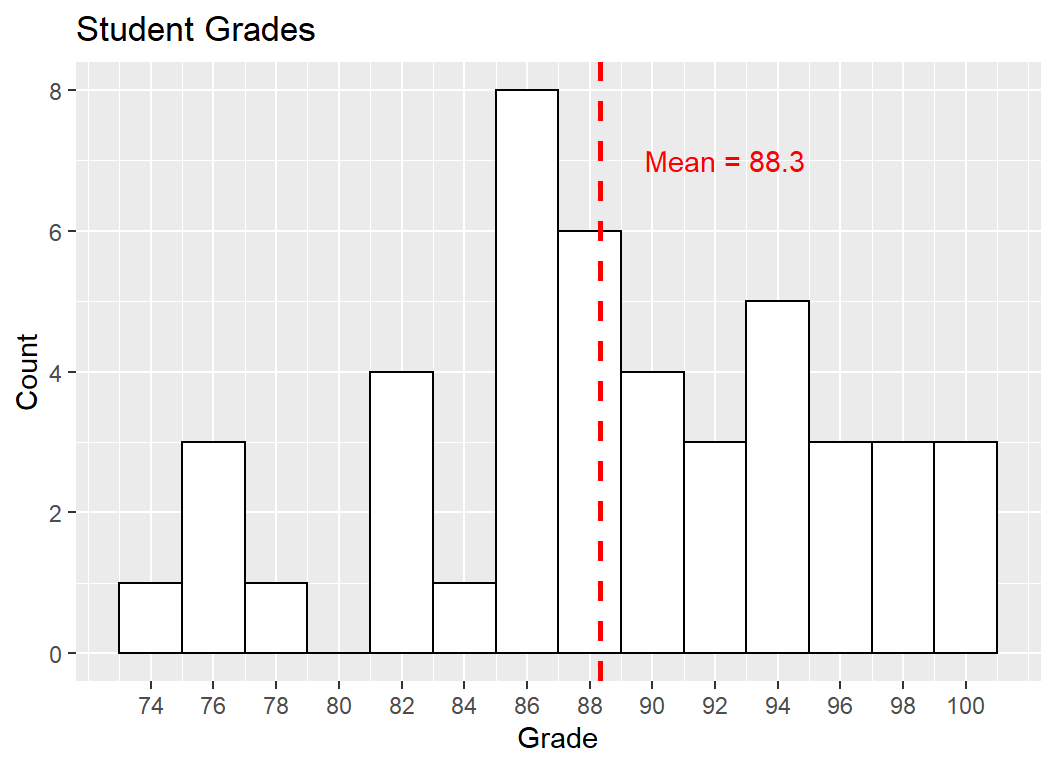
1.5 Discussion
The mean of 88.3 from the collected sample was decisive for my prediction. Since 85% was close to the maximum grade of 100, there was
a possiblity that outliers would create a left skew, lowering the mean. However, that was not the case for the sample collected. My belief about the variable and its distribution are mostly maintained by this result.
The heavy tails from the distribution was unexpected. If grades between 83 and 87 were excluded, I would be looking at a uniform distribution. This could potentially be addressed by increasing the sample size. A larger sample will also prevent outliers having a significant effect on the sample mean.
1.6 More on Chebyshev’s Inequality
Chebyshev’s inequality allows us to define an upper bound for the probability that a random variable X with unknown distribution is some distance from its expected value.
So if we set \(k=2\), the probability that \(|X - E(X)|\) lies beyond \(2\sigma\) is at most \(\frac{1}{k^2} = 0.25\). Working backwards if we start by setting \(\alpha = 0.05\), then \(\frac{1}{k^2} = 0.05\) and \(k = 4.47\). This means the probability that \(X\) falls outside of \(4.47\sigma\) is at most 0.05.
On the other hand if we knew random variable \(X\) was normally distributed, we know that exactly 95% of the data lies within +/- 1.96 standard deviations:
\[P(|X - E(X)| \geq k\sigma) = 1- 2\int_{0}^{k}\frac{1}{\sqrt{2\pi}}e^{(-\frac{1}{2}z^2)} = \alpha\]
For example: if we set \(\alpha = 0.05\), we get \(k=1.96\), which in turn states that \(|X - E(X)|\) has to be \(\geq 1.96\sigma\).
Notice how our normal distribution gives an exact probability, while chebyshev’s merely gives an upper bound. This is because chebyshev’s holds much weaker assumptions: it does not assume an underlying distribution.
Basically, the inequality states that as long as random variable \(X\) is positive and its expectation (mean) exists, the probability that \(X_i\) is greater than some value \(t\) is bound by its expectation \(E(X)\) divided by \(t\).
\(\begin{align*} E(X) & = \int_{-\infty}^{\infty}xf(x)dx && \text{definition of expectation}\\ & = \int_{-\infty}^{t}xf(x)dx + \int_{t}^{\infty}xf(x)dx && \text{expanding the integral}\\ & \geq 0 + \int_{t}^{\infty}xf(x)dx && \text{looking only at x > t}\\ & \geq t\int_{t}^{\infty}f(x)dx && \text{integrating by the lowest constant t}\\ & = tP(x \geq t) && \text{definition of probability}\\ \end{align*}\)
\(\begin{align*} & P(X \geq t) \leq \frac{E(X)}{t} && \text{markov inequality}\\ & P(|X - E(X)| \geq t) \leq \frac{E(|X - E(X)|)}{t} && \text{replace X with |X-E(X)|}\\ & P((X - E(X))^2 \geq t^2) \leq \frac{E((X - E(X))^2)}{t^2} && \text{re-apply markov inequality}\\ & P(|X - E(X)| \geq t) \leq \frac{Var(X)}{t^2}\\ & P(|\bar{X} - E(X)| \geq t) \leq \frac{Var(X)}{t^2n} && \text{for sample of more than 1}\\ \end{align*}\)
Note:
\(E(X-E(X))^2 = Var(X)\)
\(P(|X-E(X)| \geq t) = P((X-E(X))^2 \geq t^2)\)
For further reading on chebyshev’s click Here.