Chapter 2 Simulator: Before Renovation

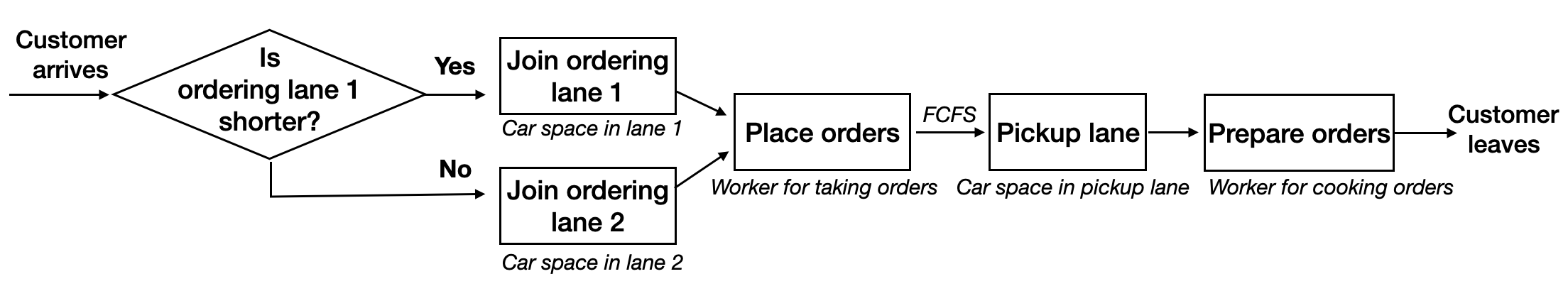
We build the DES simulator according to the following flow chart that describes the trajectory of a typical drive-thru customer. For simplicity, we utilize only two types of blocks: rectangle for Process and diamond for Decision.

Under each process block, resources required for this particular block are written in italics. For instance, when a customer places an order, a cashier worker is a system resource that takes the order. When a customer finishes ordering, he needs a car space in the pickup lane in order to proceed to the pickup station. Considering car spaces as a system resource is crucial in determining the system carline, as spatial spaces are constraining resources in drive-thru congestion.

We first load the required packages.

# Load package for discrete event simulation (DES)
library(simmer) 
library(simmer.plot)

# Load package for pipe operator %>%, which is used to call a series of functions
library(magrittr)

# For plotting
library(ggplot2)

# For data wrangling
library(reshape2)

The following block defines the model parameters, some of which can be tuned in order to evaluate the performance of various designs. For example, we can increase the number of cashiers (“num_cashier”) so as to the speed up the ordering process.

################################################################################
########### Model Parameters ###################################################
################################################################################
# time unit 1 minute
simTime = 2000

# cashier service rate
mu_cashier = 0.8

# cook service rate
mu_cook = 1/3.5

# number of cashiers
num_cashier = 2

# number of cooks
num_cook = 3

# car spaces in ordering lane
space_ordering = 200

# car spaces in pickup lane
space_pickup = 6

# Poisson arrival rate of customers
arrival_rate = 0.8

We encode a customer’s trajectory according to the flow chart.

customer = trajectory("Customer's path") %>%
  set_attribute("lane", function() {
    (get_server_count(env, "lane1")>=get_server_count(env, "lane2"))*1+1}
  ) %>% 
  select(function() {
    paste0("lane",get_attribute(env, "lane"))
  }) %>% 
  seize_selected(1) %>% # Choose the shortest ordering lane
  
  seize("cashier",amount=1) %>% # Try to seize a cashier for placing the order
  timeout(function() {rexp(1, mu_cashier)}) %>%
  release("cashier",amount=1) %>%
  
  seize("lane_pickup",amount=1) %>% # Try to seize a car space in pickup lane
  release_selected(1) %>% # Once going to the pickup lane, the customer releases the ordering lane
  
  seize("cook",amount=1) %>% # Try to seize a cook for preparing the order
  timeout(function() {rexp(1, mu_cook)}) %>%
  release("cook",amount=1) %>%
  release("lane_pickup") # After the order is ready, the car immediately leaves the system

We also define a dummy trajectory which creates a dummy entity every one unit of time. This dummy entity records the car lines at the ordering and pickup station, which will be retrieved to create the system carline metric.

dummy = trajectory() %>% # A dummy trajectory for recording the system carline
  set_attribute("carline_ordering",function() {
    carline1 = max(get_server_count(env,"lane1"),get_server_count(env,"lane2"))}) %>%
  set_attribute("carline_pickup",function() {
    carline2 = get_server_count(env,"lane_pickup")}) 

2.1 A single run

Finally, we create the simulator environment by specifying the number of resources and the arrival process. We let the simulator run for a pre-specified simulation time (“simTime’’), which is considered a single run of the drive-thru system.

env = simmer()
env %>%
  add_resource("cashier", num_cashier) %>% # Cashiers for taking orders
  add_resource("lane1", capacity=space_ordering) %>% # Ample car spaces in ordering lane1
  add_resource("lane2", capacity=space_ordering) %>% # Ample car spaces in ordering lane2
  add_resource("lane_pickup", capacity=space_pickup) %>% # Car spaces in pick up lane
  add_resource("cook", num_cook) %>% # Cooks for preparing the orders
  add_generator("Customer", customer, function() rexp(1, arrival_rate), mon=2) %>% # Customer's arrival process
  add_generator("Dummy recorder", dummy, function() 1, mon=2) %>% # Dummy trajectory records every 1 minute
  run(simTime)

After the simulator finishes running, we can retrieve all the attributes related to the dummy recorder using function. In our simulator, the “dummy” trajectory defines two attributes: the car lines at the ordering and pickup stations. Hence, the system carline is the sum of these two attributes.

############ Retrieve data from the simulator ############
############ Metric 1: System carline ################
df_att = get_mon_attributes(env)
df_att = df_att[substr(df_att$name,1,1)=='D',] # Extract values for the dummy recorder

ordering = df_att[df_att$key=="carline_ordering",'value'] # Carline at the ordering station
plot(ordering, type='l',xlab="Time (in minute)",main='Carline at the ordering station')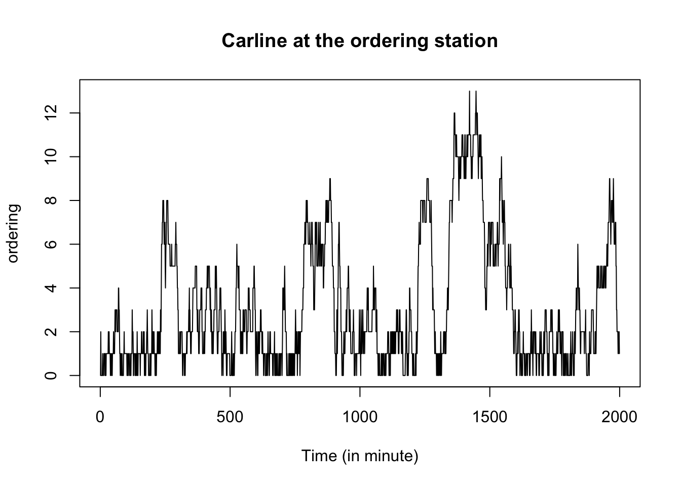

pickup = df_att[df_att$key=="carline_pickup",'value'] # Carline at the pickup station
plot(pickup, type='l',xlab="Time (in minute)",main='Carline at the pickup station')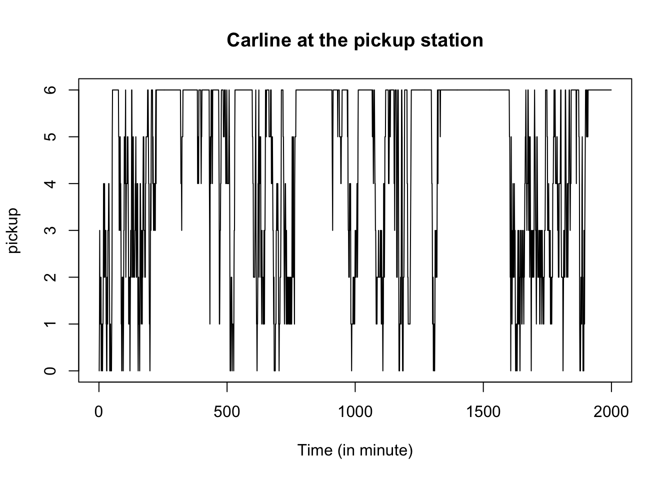

system_carline = ordering + pickup
plot(system_carline, type='l',xlab="Time (in minute)",main='System carline')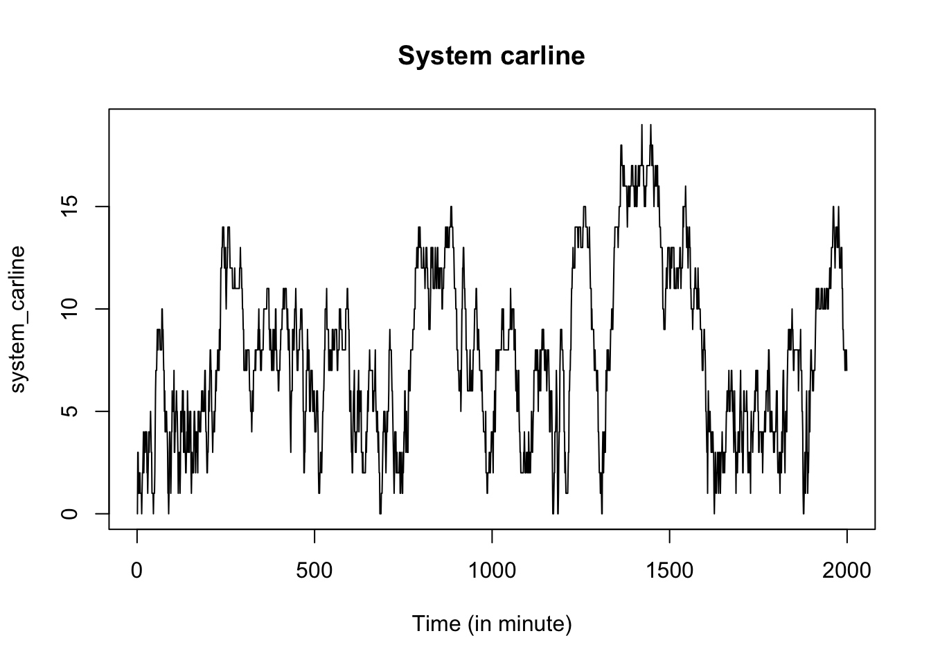

Similarly, we call function to retrieve all the data of customers’ arrivals, including individual’s arrival time and departure time. The flow time is therefore the difference between the departure and arrival time stamps.

############ Metric 2: Flow time ######################
df_arr = get_mon_arrivals(env) # All arrivals' data: including customers' and dummy recorder's
df_arr = df_arr[substr(df_arr$name,1,1)=='C',] # Extract customer's arrival data
df_arr=df_arr[order(df_arr$start_time),]

df_arr$flow_time = df_arr$end_time - df_arr$start_time

plot(df_arr$flow_time, type='l',xlab="Customer ID", ylab="Duration (in minutes)", main='Flow time of customers')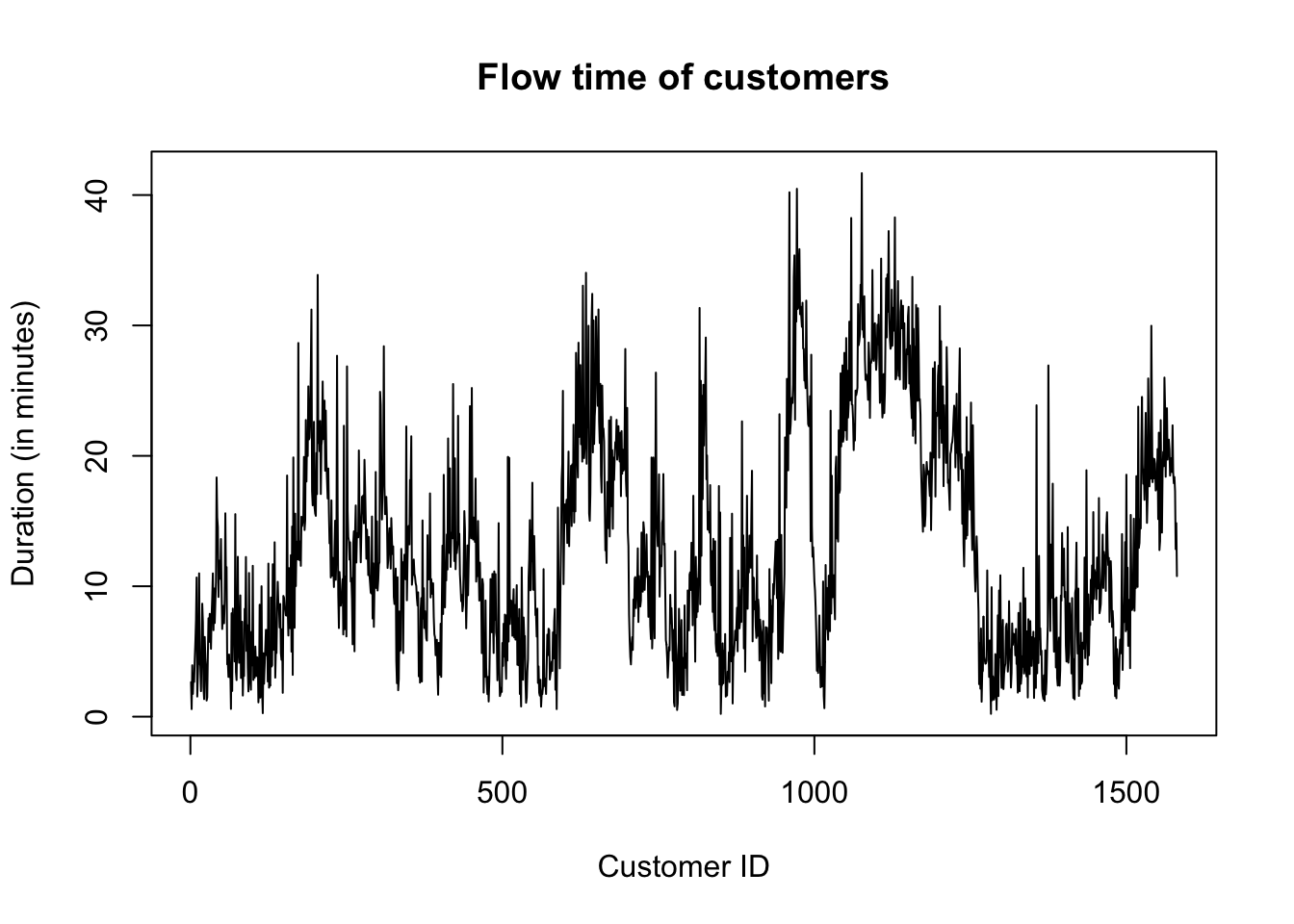

The summary statistics of the system carline and customers’ flow time are as follows. On average, the system carline is 8, and a customer spends 13 minutes in the drive-thru.

summary(system_carline)

##    Min. 1st Qu.  Median    Mean 3rd Qu.    Max. 
##   0.000   4.000   7.000   7.727  11.000  19.000

summary(df_arr$flow_time)

##    Min. 1st Qu.  Median    Mean 3rd Qu.    Max. 
##  0.2132  6.1173 10.9785 12.8596 18.7576 41.6773

2.2 Monte Carlo experiment

In order to obtain a more robust result, we next conduct a Monte Carlo experiment by repeating the single-run simulation 1000 times. In each run, we truncate the first 500 minutes when computing the average carline as the system has not reached the steady state in this initial period. Similarly, we truncate the first 200 customers when calculating the average flow time.

#####################################################################
### Monte carlo experiment ##########################################
### Create 1000 repeated simulations #################################
#####################################################################
num_rep = 1000
# Data frame for storing the performance of the Chick-fil-A before renovation
Data_before=data.frame(repetition=1:num_rep,system_carline=1:num_rep,flow_time=1:num_rep)

for(ii in 1:num_rep){
  print(paste0("Repetition ",ii))
  env = simmer()
  env %>%
    add_resource("cashier", num_cashier) %>% # 2 Cashiers for taking orders
    add_resource("lane1", capacity=space_ordering) %>% # Ample car spaces in ordering lane1
    add_resource("lane2", capacity=space_ordering) %>% # Ample car spaces in ordering lane2
    add_resource("lane_pickup", capacity=space_pickup) %>% # 6 car spaces in pick up lane
    add_resource("cook", num_cook) %>% # 3 Cooks for preparing the orders
    add_generator("Customer", customer, function() rexp(1, arrival_rate), mon=2) %>% # Customer's arrival process
    add_generator("Dummy recorder", dummy, function() 1, mon=2) %>% # Dummy trajectory records every 1 minute
    run(simTime)
  
  ## average system carline length
  df_att = get_mon_attributes(env)
  df_att = df_att[substr(df_att$name,1,1)=='D',] # only look at dummy recorder
  ordering = df_att[df_att$key=="carline_ordering",'value']
  
  pickup = df_att[df_att$key=="carline_pickup",'value']
  
  system_carline = ordering + pickup
  
  Data_before[ii,'system_carline']=mean(system_carline[500:length(system_carline)])
  
  ## average flow time
  df_arr = get_mon_arrivals(env)
  df_arr = df_arr[substr(df_arr$name,1,1)=='C',] # picking customer's data only
  
  df_arr$flow_time = df_arr$end_time - df_arr$start_time
  
  Data_before[ii,'flow_time']=mean(df_arr$flow_time[200:nrow(df_arr)]) 
}

The following Figure shows the distribution of the average system carline across all 1000 runs. The mean is around 11, and the long tail suggests the possibility of extreme traffic congestion in the Chick-fil-A drive-thru.

ggplot(Data_before,aes(x=system_carline)) + geom_density() + theme_bw() +
   geom_vline(aes(xintercept=mean(system_carline)),
            color="blue", linetype="dashed", linewidth=1)+
  labs(title="Distribution of the average system carline",x="System carline", y = "Density")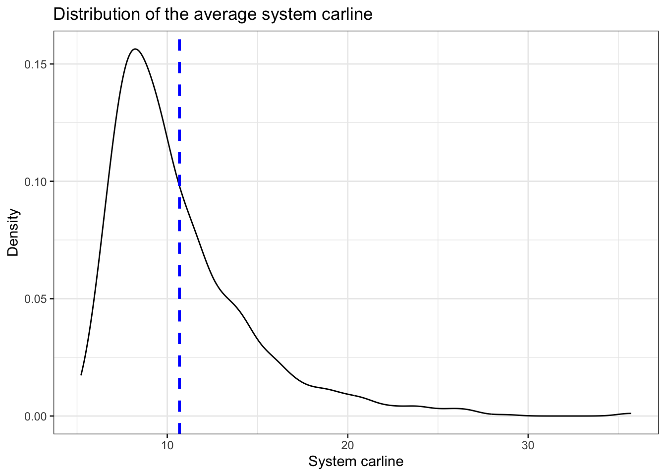

The distribution of the average flow time follows a similar pattern. Though the mean wait is around 19 minutes, some customers may spend significantly longer time due to the potential extreme congestion.

ggplot(Data_before,aes(x=flow_time)) + geom_density() + theme_bw() +
   geom_vline(aes(xintercept=mean(flow_time)),
            color="blue", linetype="dashed", linewidth=1)+
  labs(title="Distribution of the average flow time",x="Flow time", y = "Density")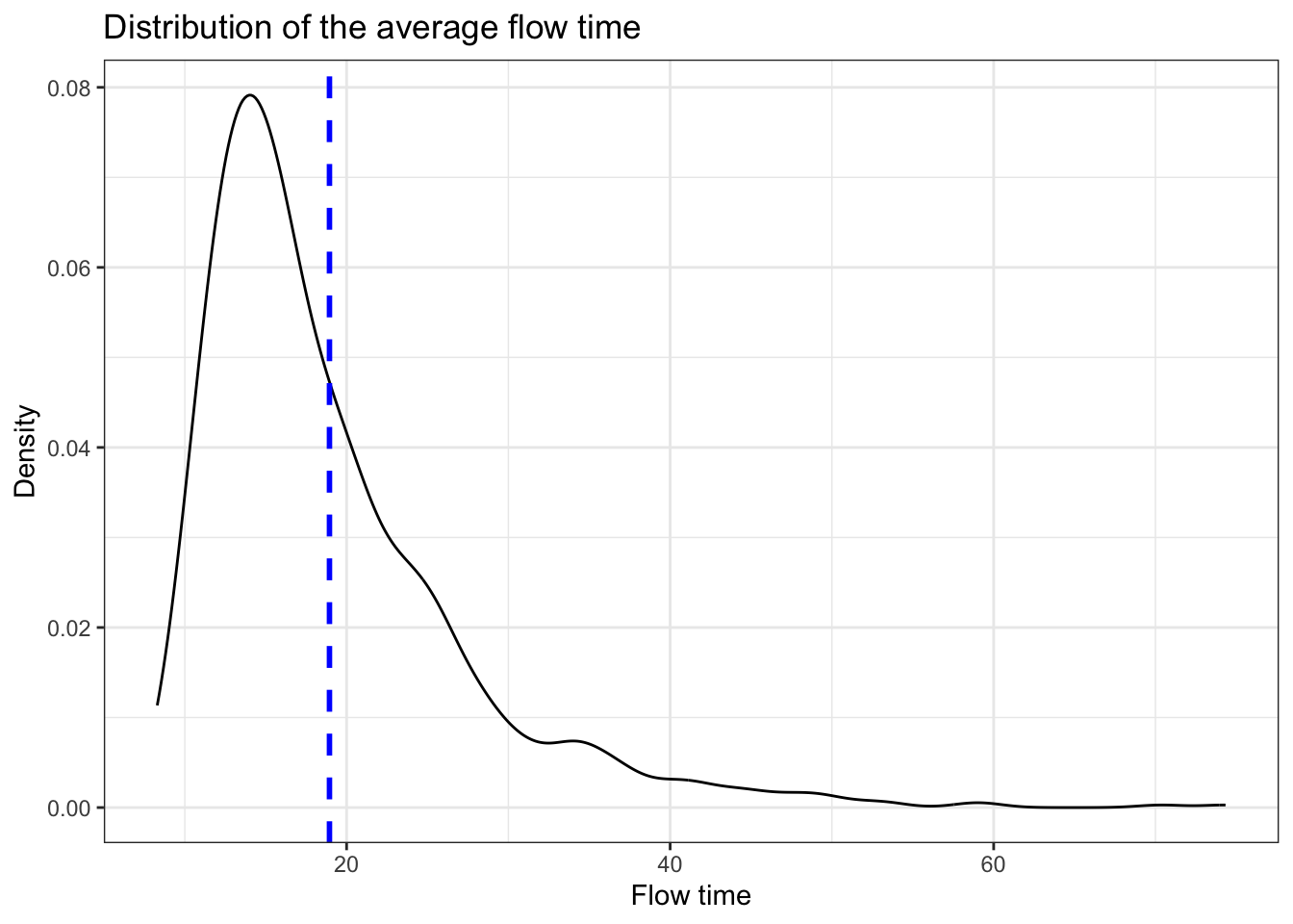

# Summary statistcis: System carline
summary(Data_before$system_carline)

##    Min. 1st Qu.  Median    Mean 3rd Qu.    Max. 
##   5.219   7.929   9.539  10.675  12.207  35.709

# Summary statistcis: Flow time
summary(Data_before$flow_time)

##    Min. 1st Qu.  Median    Mean 3rd Qu.    Max. 
##   8.294  13.473  16.594  18.941  22.003  74.332