Chapter 3 Simulator: After Renovation

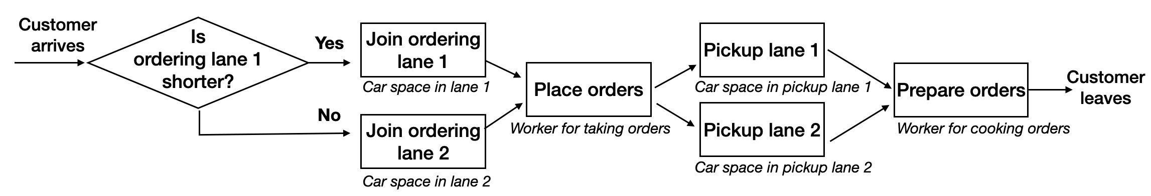
After renovation, the key difference in the flow chart is an additional pickup lane with extra car spaces.

Thus, we redefine the model parameters as follows.

################################################################################
########### Model Parameters ###################################################
################################################################################
# time unit 1 minute
simTime = 2000

# cashier service rate
mu_cashier = 0.8

# cook service rate
mu_cook = 1/3.5 

# number of cashiers
num_cashier = 2

# number of cooks
num_cook = 3

# car spaces in ordering lane
space_ordering = 200

# car spaces in each pickup lane
space_pickup = 10

# Poisson arrival rate of customers
arrival_rate = 0.8 

In the customer’s trajectory, the car will move from the ordering lane to its corresponding pickup lane instead of merging into a single pickup lane.

customer = trajectory("Customer's path") %>%
  set_attribute("lane", function() {
    (get_server_count(env, "lane1")>=get_server_count(env, "lane2"))*1+1}
  ) %>% 
  select(function() {
    paste0("lane",get_attribute(env, "lane"))
  }) %>% 
  seize_selected(1) %>% # Choose the shortest ordering lane
  
  seize("cashier",amount=1) %>% # Try to seize a cashier for placing the order
  timeout(function() {rexp(1, mu_cashier)}) %>%
  release("cashier",amount=1) %>%
  
  select(function() {ifelse(get_attribute(env, "lane")==1,"lane1pickup","lane2pickup")}, id=2) %>% 
  seize_selected(amount=1, id=2) %>% # Try to go on to the corresponding pickup lane
  release_selected(1) %>% # Once going to the pickup lane, release the ordering lane
  
  seize("cook",amount=1) %>% # Try to seize a cook for preparing the order
  timeout(function() {rexp(1, mu_cook)}) %>%
  release("cook",amount=1) %>%
  release_selected(amount=1, id=2) # After the order is ready, the car immediately leaves the system

dummy = trajectory() %>% # A dummy trajectory for recording the system carline of lane1 and lane2
  set_attribute("carline_lane1",function() {
    carline1 = get_server_count(env,"lane1")+get_server_count(env,"lane1pickup")}) %>%
  set_attribute("carline_lane2",function() {
    carline2 = get_server_count(env,"lane2")+get_server_count(env,"lane2pickup")})  

3.1 A single run

We first implement a single run of the after-renovation simulator.

env = simmer()
env %>%
  add_resource("cashier", num_cashier) %>% # 2 Cashiers for taking orders
  add_resource("lane1", capacity=space_ordering) %>% # Ample car spaces in ordering lane1
  add_resource("lane2", capacity=space_ordering) %>% # Ample car spaces in ordering lane2
  add_resource("lane1pickup", capacity=space_pickup) %>% # Car spaces in pick up lane1
  add_resource("lane2pickup", capacity=space_pickup) %>% # Car spaces in pick up lane2
  add_resource("cook", num_cook) %>% # 3 Cooks for preparing the orders
  add_generator("Customer", customer, function() rexp(1, arrival_rate), mon=2) %>% # Customer's arrival process
  add_generator("Dummy recorder", dummy, function() 1, mon=2) %>% # Dummy trajectory records every 1 minute
  run(simTime)

## simmer environment: anonymous | now: 2000 | next: 2000
## { Monitor: in memory }
## { Resource: cashier | monitored: TRUE | server status: 1(2) | queue status: 0(Inf) }
## { Resource: lane1 | monitored: TRUE | server status: 0(200) | queue status: 0(Inf) }
## { Resource: lane2 | monitored: TRUE | server status: 1(200) | queue status: 0(Inf) }
## { Resource: lane1pickup | monitored: TRUE | server status: 3(10) | queue status: 0(Inf) }
## { Resource: lane2pickup | monitored: TRUE | server status: 4(10) | queue status: 0(Inf) }
## { Resource: cook | monitored: TRUE | server status: 3(3) | queue status: 4(Inf) }
## { Source: Customer | monitored: 2 | n_generated: 1590 }
## { Source: Dummy recorder | monitored: 2 | n_generated: 2000 }

Similarly to the previous experiment, we retrieve the simulation data to compute the system performance.

############ Retrieve data from the simulator ############
############ Metric 1: System carline ################
df_att = get_mon_attributes(env)
df_att = df_att[substr(df_att$name,1,1)=='D',] # Extract values for the dummy recorder
carline1 = df_att[df_att$key=='carline_lane1',] 
carline2 = df_att[df_att$key=='carline_lane2',] 
system_carline = pmax(carline1$value,carline2$value)

plot(system_carline, type='l',xlab="Time (in minute)",main='System carline')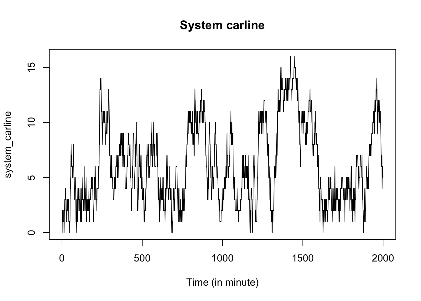

############ Metric 2: Flow time ######################
df_arr = get_mon_arrivals(env) # All arrivals' data: including customers' and dummy recorder's
df_arr = df_arr[substr(df_arr$name,1,1)=='C',] # Extract customer's arrival data

df_arr$flow_time = df_arr$end_time - df_arr$start_time

plot(df_arr$flow_time, type='l',xlab="Customer ID", ylab="Duration (in minutes)", main='Flow time of customers')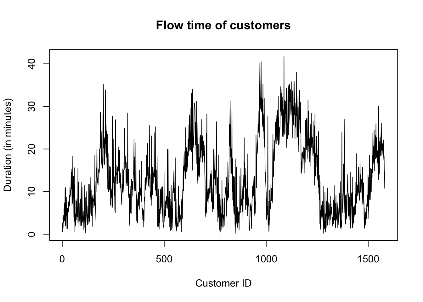

The summary statistics below suggest that after renovation, the system carline reduces from 8 to 6, but the flow time remains 13 minutes.

summary(system_carline)

##    Min. 1st Qu.  Median    Mean 3rd Qu.    Max. 
##   0.000   3.000   5.000   6.149   9.000  16.000

summary(df_arr$flow_time)

##    Min. 1st Qu.  Median    Mean 3rd Qu.    Max. 
##  0.2132  6.1173 10.9864 12.8596 18.6320 41.6773

3.2 Monte Carlo experiment

Now, we repeat the single-run experiment 1000 times to compute a robust measurement of system performances.

#####################################################################
### Monte carlo experiment ##########################################
### Create num_rep repeated simulations #################################
#####################################################################

# Data frame for storing the performance of the Chick-fil-A after renovation
num_rep = 1000
Data_after=data.frame(repetition=1:num_rep,system_carline=1:num_rep,flow_time=1:num_rep)

for(ii in 1:num_rep){
  print(paste0("Repetition ",ii))
  env = simmer()
  env %>%
    add_resource("cashier", num_cashier) %>% # Cashiers for taking orders
    add_resource("lane1", capacity=space_ordering) %>% # Ample car spaces in ordering lane1
    add_resource("lane2", capacity=space_ordering) %>% # Ample car spaces in ordering lane2
    add_resource("lane1pickup", capacity=space_pickup) %>% # Car spaces in pick up lane1
    add_resource("lane2pickup", capacity=space_pickup) %>% # Car spaces in pick up lane2
    add_resource("cook", num_cook) %>% # 3 Cooks for preparing the orders
    add_generator("Customer", customer, function() rexp(1, arrival_rate), mon=2) %>% # Customer's arrival process
    add_generator("Dummy recorder", dummy, function() 1, mon=2) %>% # Dummy trajectory records every 1 minute
    run(simTime)
  
  ## average system carline length
  df_att = get_mon_attributes(env)
  df_att = df_att[substr(df_att$name,1,1)=='D',] # Extract values for the dummy recorder
  carline1 = df_att[df_att$key=='carline_lane1',] 
  carline2 = df_att[df_att$key=='carline_lane2',] 
  system_carline = pmax(carline1$value,carline2$value)
  
  Data_after[ii,'system_carline']=mean(system_carline[500:length(system_carline)])
  
  ## average flow time
  df_arr = get_mon_arrivals(env)
  df_arr = df_arr[substr(df_arr$name,1,1)=='C',] # picking customer's data only
  
  df_arr$flow_time = df_arr$end_time - df_arr$start_time
  
  Data_after[ii,'flow_time']=mean(df_arr$flow_time[200:nrow(df_arr)]) 
}

The following Figure shows the distributions of the average system carline and the average flow time across all 1000 runs.

ggplot(Data_after,aes(x=system_carline)) + geom_density() + theme_bw() +
   geom_vline(aes(xintercept=mean(system_carline)),
            color="blue", linetype="dashed", linewidth=1)+
  labs(title="Distribution of the average system carline",x="System carline", y = "Density")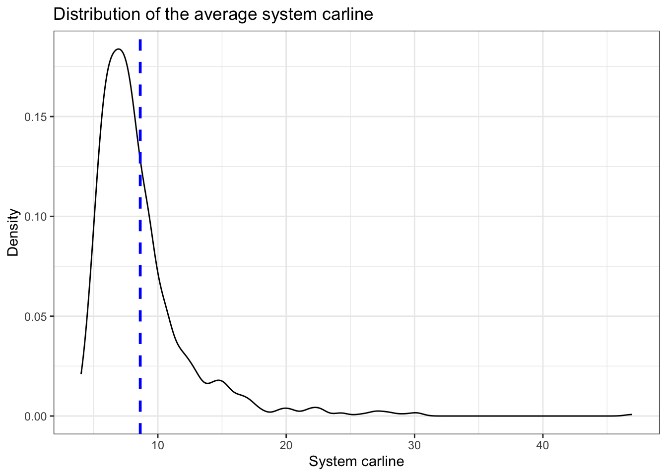

ggplot(Data_after,aes(x=flow_time)) + geom_density() + theme_bw() +
   geom_vline(aes(xintercept=mean(flow_time)),
            color="blue", linetype="dashed", linewidth=1)+
  labs(title="Distribution of the average flow time",x="Flow time", y = "Density")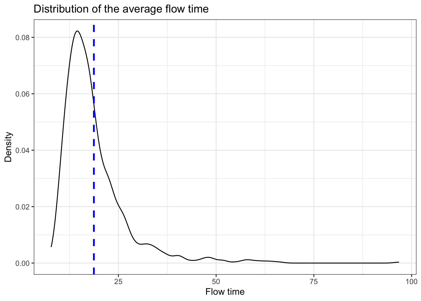

3.3 Evaluate the impact of Chick-fil-A renovation

We now compare the metrics of two simulators to understand the impact of Chick-fil-A renovation on its drive-thru congestion. Specifically, we plot the distributions of the flow time and the system carline as follows.

Data_before$facility = 'Before renovation'
Data_after$facility = 'After renovation'

Data = rbind(Data_before,Data_after)

ggplot(Data, aes(x=system_carline,lty=facility)) +
  geom_density(linewidth=0.7)+
  labs(title="Distribution of the average system carline",x="System carline", y = "Density")+
  scale_linetype_discrete(name="Chick-fil-A facility")+
  theme_bw()+
  theme(text=element_text(size=15))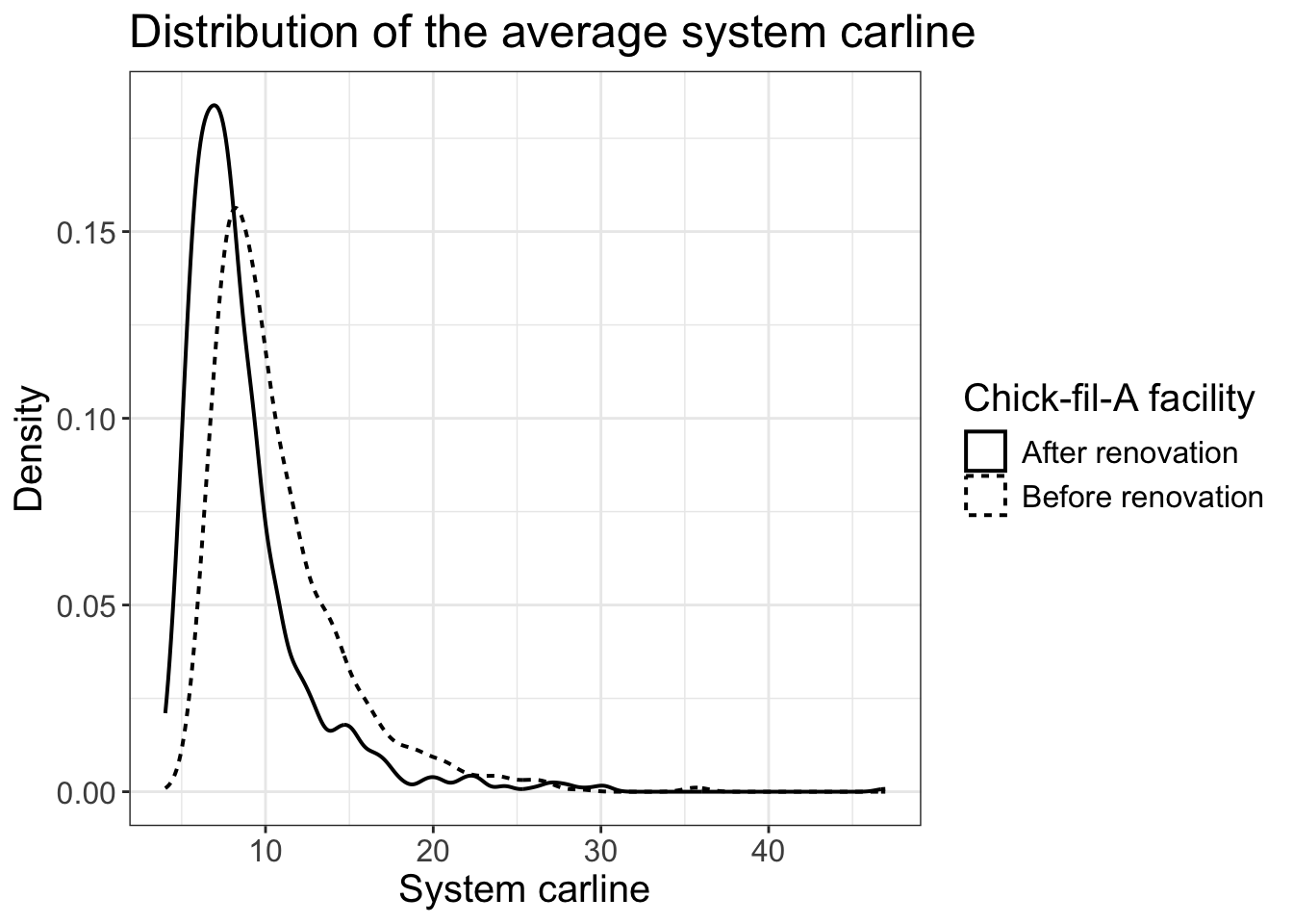

ggplot(Data, aes(x=flow_time,lty=facility)) +
  geom_density(linewidth=0.7)+
  labs(title="Distribution of the average flow time",x="Flow time", y = "Density")+
  scale_linetype_discrete(name="Chick-fil-A facility")+
  theme_bw()+
  theme(text=element_text(size=15))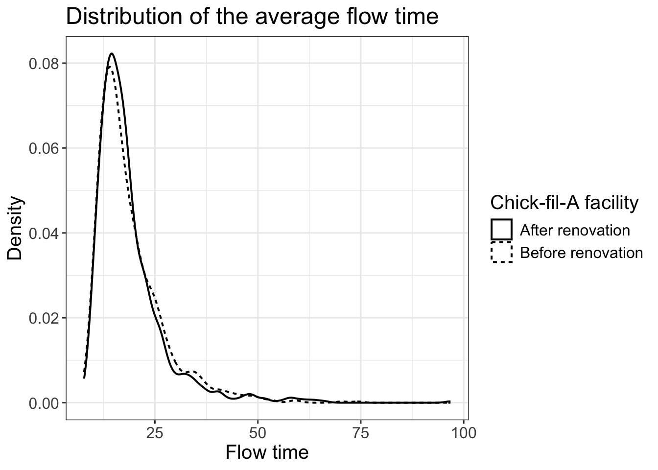

Compared with the metrics before the renovation, the average system carline of the new facility is reduced by 20%, but the average flow time is almost identical. In other words, Chick-fil-A’s new design is ineffective in reducing customers’ waiting time! A formal t-test also suggests that the reduction in the system carline is significant, but flow time distributions before and after the renovation show no significant difference.

This result highlights that without a rigorous analysis of bottleneck resources, some costly measures, such as a large-scale renovation, may not have any impact in reducing congestion. Therefore, the next module discusses bottleneck analysis, which identifies the scarce resource in the customer’s trajectory that causes long queues in the whole chain. Identifying bottlenecks is crucial in determining which resources the business should prioritize when making investments to improve overall efficiency.