15 Data Manipulation (IV)
This chapter discusses another technique in data frame manipulations, reshaping data frames from wide to long format or from long to wide format.
15.1 Wide and long formats
The term reshape points to something very specific in data frame manipulation, which is to restructure a data frame from wide to long format or from long to wide format.
What exactly does wide or long mean for a data frame? How do data frames in wide or long format looks like? Actually, we have some good examples from our Yahoo Finance datasets.
wide
When we download historical stocks data from Yahoo Finance using quantmod, we will see that information for each stock is stored in individual objects.
library(quantmod)
tickers <- c("AFL","AAPL", "MMM")
getSymbols(tickers, src = "yahoo",
           from = "2021-01-01",
           to = "2021-01-31")
## MMM.Open MMM.High MMM.Low MMM.Close MMM.Volume MMM.Adjusted
## 2021-01-04 175.00 176.20 170.55 171.87 2996200 169.2200
## 2021-01-05 172.01 173.25 170.65 171.58 2295300 168.9345
## 2021-01-06 172.72 175.57 172.04 174.19 3346400 171.5043
## 2021-01-07 171.56 173.46 166.16 169.72 5863400 167.1032
## 2021-01-08 169.17 169.54 164.61 166.62 4808100 164.0510
## 2021-01-11 166.10 167.14 165.00 165.20 2736600 162.6529These are xts objects.
## [1] "xts" "zoo"An xts object can be thought of as a matrix of observations combined with an index of corresponding dates and times: xts = matrix + times. The index holds the information that we need for xts to treat our data as a time series.
These time series objects are designed to be bound together by dates and times. If we combine these xts objects, we bind these data frames horizontally.
##            AAPL.Open AAPL.High AAPL.Low AAPL.Close AAPL.Volume AAPL.Adjusted AFL.Open
## 2021-01-04    133.52    133.61   126.76     129.41   143301900      128.9978    44.60
## 2021-01-05    128.89    131.74   128.43     131.01    97664900      130.5927    43.33
## 2021-01-06    127.72    131.05   126.38     126.60   155088000      126.1967    43.91
## 2021-01-07    128.36    131.63   127.86     130.92   109578200      130.5030    45.18
## 2021-01-08    132.43    132.63   130.23     132.05   105158200      131.6294    44.92
## 2021-01-11    129.19    130.17   128.50     128.98   100384500      128.5692    44.22
##            AFL.High AFL.Low AFL.Close AFL.Volume AFL.Adjusted MMM.Open MMM.High
## 2021-01-04    44.70   43.03     43.19    3111200     42.63539   175.00   176.20
## 2021-01-05    43.70   42.96     43.26    2561700     42.70449   172.01   173.25
## 2021-01-06    45.20   43.54     44.93    3842900     44.35305   172.72   175.57
## 2021-01-07    45.26   44.45     44.68    4217400     44.10626   171.56   173.46
## 2021-01-08    44.99   43.72     44.49    2915700     43.91870   169.17   169.54
## 2021-01-11    44.82   44.00     44.51    2479000     43.93844   166.10   167.14
##            MMM.Low MMM.Close MMM.Volume MMM.Adjusted
## 2021-01-04  170.55    171.87    2996200     169.2200
## 2021-01-05  170.65    171.58    2295300     168.9345
## 2021-01-06  172.04    174.19    3346400     171.5043
## 2021-01-07  166.16    169.72    5863400     167.1032
## 2021-01-08  164.61    166.62    4808100     164.0510
## 2021-01-11  165.00    165.20    2736600     162.6529
The resulting data frame is wide. In this wide format, we have one record for each date. Prices for different stocks on the same date will be in one row. The observations for different stocks are coded as different columns.
long
Compare what we get from quantmod with what we get from tidyquant.
library(tidyquant)
tq <- tq_get(c("AFL","AAPL", "MMM"),
             get = "stock.prices",
             from="2021-01-01",to="2021-01-31")
We get a data frame that stores information of all the stocks vertically. The resulting data frame is long.
## # A tibble: 11 × 8
##    symbol date        open  high   low close    volume adjusted
##    <chr>  <date>     <dbl> <dbl> <dbl> <dbl>     <dbl>    <dbl>
##  1 AFL    2021-01-25  46.0  46.6  45.7  46.6   5031400     46.0
##  2 AFL    2021-01-26  46.7  47.0  46.4  46.4   3956600     45.8
##  3 AFL    2021-01-27  45.8  46.1  44.8  45.2   4463200     44.6
##  4 AFL    2021-01-28  45.6  46.5  45.3  46.1   4272600     45.5
##  5 AFL    2021-01-29  45.9  46.0  44.8  45.2   5236800     44.6
##  6 AAPL   2021-01-04 134.  134.  127.  129.  143301900    129.
##  7 AAPL   2021-01-05 129.  132.  128.  131.   97664900    131.
##  8 AAPL   2021-01-06 128.  131.  126.  127.  155088000    126.
##  9 AAPL   2021-01-07 128.  132.  128.  131.  109578200    131.
## 10 AAPL   2021-01-08 132.  133.  130.  132.  105158200    132.
## 11 AAPL   2021-01-11 129.  130.  128.  129.  100384500    129.
In this long format, in each record, the variable date records the time period, and the variable symbol groups the records from the same stocks. There will be multiple records for each date. Each row is one time point per stock.
wide or long
Both formats have their advantages. If the data is collected on the same time points, the wide format has no redundancy or repetition. Stock prices collected on the same day take one row. Elementary statistical computations are easy to do in the wide format.
The long format, on the other hand, has an explicit time variable available that can be used for analysis. Graphs and statistical analyses are easier in the long format.
15.2 Reshaping data frames from long to wide
The next question is how to convert between wide and the long formats.
First, long to wide. For instance, how can we convert the long dataset collected by tidyquant to the wide format? The package tidyr offers the function pivot_wider() that can help us convert a data frame from long to wide in most situations that are not hugely complicated.
library(tidyr)
tq_to_wide <-
  tq %>%
  pivot_wider(names_from = symbol,
              values_from = c(open,close,high,low,volume,adjusted),
              names_sep = ".")
Arguments names_from and values_from are a pair of arguments describing which column(s) to get the name of the output column (names_from), and which column(s) to get the cell values from (values_from).
If values_from contains multiple values, the value will be added to the beginning of the output column. Therefore, the variable symbol in the original long format would be added to the price variables open, close, high, low, volume, and adjusted.
## # A tibble: 6 × 19
##   date       open.AFL open.AAPL open.MMM close.AFL close.AAPL close.MMM high.AFL
##   <date>        <dbl>     <dbl>    <dbl>     <dbl>      <dbl>     <dbl>    <dbl>
## 1 2021-01-04     44.6      134.     175       43.2       129.      172.     44.7
## 2 2021-01-05     43.3      129.     172.      43.3       131.      172.     43.7
## 3 2021-01-06     43.9      128.     173.      44.9       127.      174.     45.2
## 4 2021-01-07     45.2      128.     172.      44.7       131.      170.     45.3
## 5 2021-01-08     44.9      132.     169.      44.5       132.      167.     45.0
## 6 2021-01-11     44.2      129.     166.      44.5       129.      165.     44.8
## # ℹ 11 more variables: high.AAPL <dbl>, high.MMM <dbl>, low.AFL <dbl>, low.AAPL <dbl>,
## #   low.MMM <dbl>, volume.AFL <dbl>, volume.AAPL <dbl>, volume.MMM <dbl>,
## #   adjusted.AFL <dbl>, adjusted.AAPL <dbl>, adjusted.MMM <dbl>
Because we have multiple variables here, these column names need to be joined together by a pattern, which is a dot. This is specified in names_sep.
15.3 Reshaping data frames from wide to long
tidyr has also provides a function pivot_longer() to convert a data frame from wide to long.
Let’s discuss a more meaningful application of reshaping a data frame from wide to long for visualization. The task is to make a line graph with multiple lines using our stocks dataset.
We created a subset where it only contains data of the company MMM . We also created a new variable SMA_2 that is the simple moving average for the past two days. The plot with a single line looks like this.
library(dplyr)
library(ggplot2)

sp500 %>%
  mutate(SMA_2 = SMA(close, n = 2)) %>%
  filter(symbol == "MMM") %>%
  ggplot(aes(x = date, y = SMA_2)) +
    geom_line() +
    geom_point()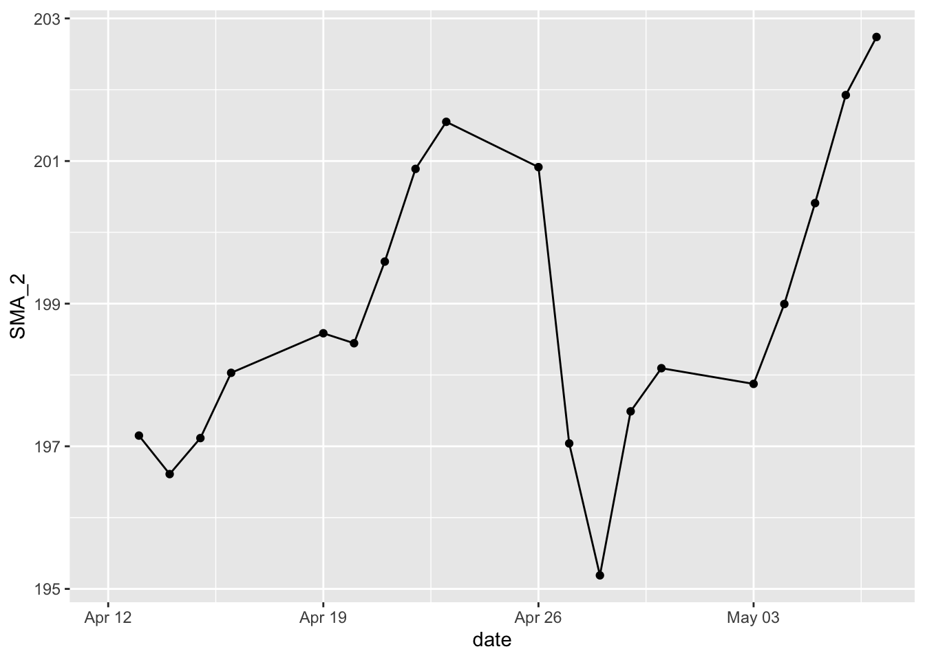
We’ll explain how to visualize data with R later, and focus on the motivation of reshaping the dataset for our visualization task.
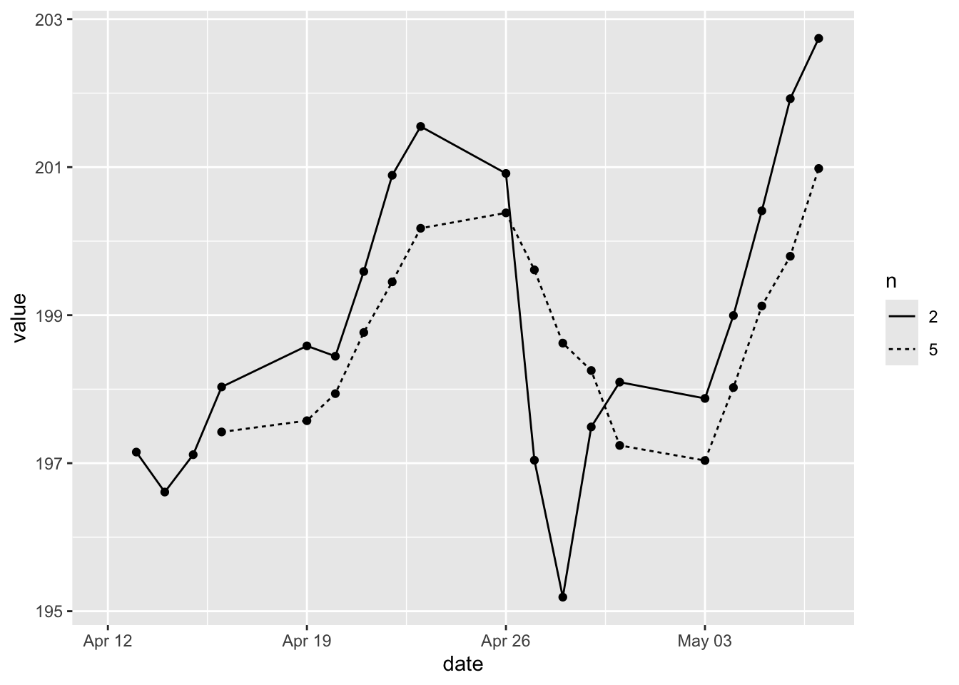
If we want to add a new line of the simple moving average for the past five days, we need to create a new subset, where we have an additional column of the SMA for the past five days.
sp500 %>%
  mutate(SMA_2 = SMA(close, n = 2)) %>%
  mutate(SMA_5 = SMA(close, n = 5)) %>%
  filter(symbol == "MMM") %>%
  select(symbol, date, SMA_2, SMA_5)
## # A tibble: 20 × 4
## symbol date SMA_2 SMA_5
## <chr> <date> <dbl> <dbl>
## 1 MMM 2021-04-12 NA NA
## 2 MMM 2021-04-13 197. NA
## 3 MMM 2021-04-14 197. NA
## 4 MMM 2021-04-15 197. NA
## 5 MMM 2021-04-16 198. 197.
## 6 MMM 2021-04-19 199. 198.
## 7 MMM 2021-04-20 198. 198.
## 8 MMM 2021-04-21 200. 199.
## 9 MMM 2021-04-22 201. 199.
## 10 MMM 2021-04-23 202. 200.
## 11 MMM 2021-04-26 201. 200.
## 12 MMM 2021-04-27 197. 200.
## 13 MMM 2021-04-28 195. 199.
## 14 MMM 2021-04-29 197. 198.
## 15 MMM 2021-04-30 198. 197.
## 16 MMM 2021-05-03 198. 197.
## 17 MMM 2021-05-04 199. 198.
## 18 MMM 2021-05-05 200. 199.
## 19 MMM 2021-05-06 202. 200.
## 20 MMM 2021-05-07 203. 201.However, for visualization, we need a column that contains both SMAs for the past two days and for past five days.
ggplot(aes(x = date, y = SMA_2_5, linetype = n)) +
    geom_line() +
    geom_point()
In other words, we need the dataset to be of the long format, where the two groups are in one column. We can convert the wide format to the long format using the function pivot_longer() from tidyr.
MMM_SMA <-
  sp500 %>%
  mutate(SMA_2 = SMA(close, n = 2)) %>%
  mutate(SMA_5 = SMA(close, n = 5)) %>%
  filter(symbol == "MMM") %>%
  select(symbol, date, SMA_2, SMA_5) %>%
  pivot_longer(cols = SMA_2:SMA_5,
               names_to = c("SMA", "n"),
               names_pattern = "(.)_(.)")
In pivot_longer(), cols specifies the columns to pivot into longer format. names_to is a character vector that specifies the names of the columns to create. names_pattern controls how the column name would be broken up if we have multiple variable names. It takes a regular expression containing matching groups.
## # A tibble: 40 × 5
##    symbol date       SMA   n     value
##    <chr>  <date>     <chr> <chr> <dbl>
##  1 MMM    2021-04-12 A     2       NA
##  2 MMM    2021-04-12 A     5       NA
##  3 MMM    2021-04-13 A     2      197.
##  4 MMM    2021-04-13 A     5       NA
##  5 MMM    2021-04-14 A     2      197.
##  6 MMM    2021-04-14 A     5       NA
##  7 MMM    2021-04-15 A     2      197.
##  8 MMM    2021-04-15 A     5       NA
##  9 MMM    2021-04-16 A     2      198.
## 10 MMM    2021-04-16 A     5      197.
## # ℹ 30 more rows
As shown above, the two SMAs now both go to the column value. There are some missing values here because we are running an SMA for the past n days. For n-1 days, SMAs will be missing.
Now we can create a line graph by group.