Chapter 3 Spatial Models on Lattices
Instead of continuous index set considered in Part 1, this part is concerned with the situation where the index set \(D\) is a countable collection of spatial sites at which data are observed. The collection \(D\) of such sites is called a lattice, which is then supplemented with neighborhood information.
3.1 Lattices
Latices
Lattice refers to a countable collection of (spatial) sites, either spatially regular or irregular.
Set Sudden Infant Death Syndrome (SIDS) in North Carolina, 1974-1978 as an example. The lattice form of the data can be drawn as Figure 3.1.
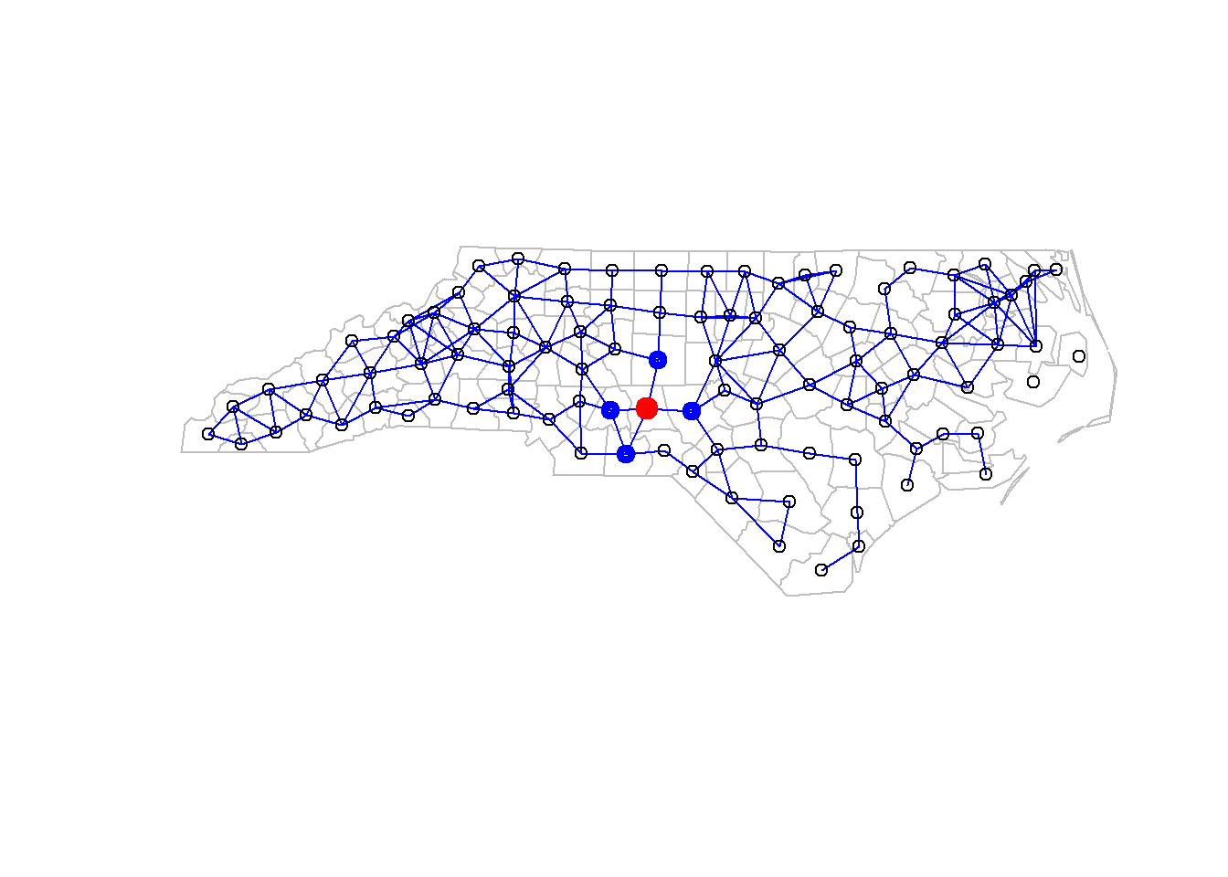
Figure 3.1: Lattice Figure of Sudden Infant Death Syndrome (SIDS) in North Carolina, 1974-1978
Neighborhoods
A site \(k\) is defined to be a neighbor of site \(i\) if the conditional distribution of \(Z\left(s_{i}\right)\), given all other site values, depends functionally on \(z\left(s_{k}\right)\), for \(k \neq i\). Also define \[\begin{equation} N_{i} \equiv\{k: k \text { is a neighbor of } i\} \tag{3.1} \end{equation}\] to be the neighborhood set of site \(i\).
Neighborhoods is important in lattice data. In SIDS data example, neighborhood relationships are drawn by blue line in Figure 3.1.Here, counties whose seats are closer than 30 miles are deemed neighbors. For instance, if we consider the bold red points, four blue points around it are neighbors.
3.2 Spatial Models for Lattice Data
In spatial domain, the conditional approach 3.2.2 and the simultaneous approach 3.2.1 result in different models.
3.2.1 Simultaneous Spatial Models
3.2.1.1 General Form
For simplicity, consider the square lattice in the plane \(\mathbb{R}^2\). \[\begin{equation} D=\{s=(u, v): u=\ldots,-2,-1,0,1,2, \ldots ; v=\ldots,-2,-1,0,1,2, \ldots\} \tag{3.2} \end{equation}\]
The joint approach is to assume \[\begin{equation} \operatorname{Pr}(\mathbf{z})=\prod_{(u, v) \in D} Q_{u v}(z(u, v) ; z(u-1, v), z(u+1, v), z(u, v-1), z(u, v+1)). \tag{3.3} \end{equation}\]
Equation (3.3) suggests that the probability of values on a specific location is determined by values of its neighbors.
Model definition of simultaneous spatial models \[\begin{equation} \phi\left(T_{1}, T_{2}\right) Z(u, v)=\epsilon(u, v) \tag{3.4} \end{equation}\] where \[\begin{equation} \left\{\begin{aligned} & T_{1} Z(u, v)=Z(u+1, v) \\ & T_{1}^{-1} Z(u, v)=Z(u-1, v) \\ & T_{2} Z(u, v)=Z(u, v+1) \\ & T_{2}^{-1} Z(u, v)=Z(u, v-1) \end{aligned} \right. \tag{3.5} \end{equation}\] and \[\begin{equation} \phi\left(T_{1}, T_{2}\right)=\sum_{i} \sum_{j} a_{i j} T_{1}^{i} T_{2}^{j} \tag{3.6} \end{equation}\]
Notice that \(\phi(c_1, c_2)\neq 0\) for any complex number \(|c_1| = |c_2| = 1\) must be met to ensure obtaining a stationary process.
3.2.1.2 Simultaneously Specified Spatial Gaussian Models
For this section, assume that \(\{Z(s): s \in D\}=\left\{Z\left(s_{i}\right): i=1, \ldots, n\right\}\) is defined on a finite subset of the integer lattice in the plane.
Suppose \(\boldsymbol{\epsilon}=\left(\epsilon\left(s_{1}\right), \ldots, \epsilon\left(s_{n}\right)\right) \sim \operatorname{Gua}(0, \Lambda)\), where \(\Lambda=\sigma^{2} I\) and \(B=\left(b_{i j}\right)\), where \(b_{ij} = 0\) means \(s_1, s_2\) are independent. If \(I - B\) is invertable, then simultaneously specified spatial gaussian model is writen as \[\begin{equation} (I-B)(\mathbf{Z}-\mu)=\epsilon \tag{3.7} \end{equation}\] Equally, \[\begin{equation} Z\left(s_{i}\right)=\mu_{i}+\sum_{j=1}^{n} b_{i j}\left(Z\left(s_{j}\right)-\mu_{j}\right)+\epsilon_{i} \tag{3.8} \end{equation}\]
- From equation (3.7), we have \(\mathbf{Z} \sim \operatorname{Gau}\left(\mu,(I-B)^{-1} \Lambda\left(I-B^{\top}\right)^{-1}\right)\).
- Equation (3.8), this is a spatial analogue of the autoregressive model.
- Note that \(\left.\left.\operatorname{Cov}(\boldsymbol{\epsilon}, \mathbf{Z})=\operatorname{cov}\left(\boldsymbol{\epsilon},(I-B)^{-1}\right) \boldsymbol{\epsilon}\right)=\Lambda\left(I-B^{\top}\right)^{-1}\right)\) is not diagonal, which means the error is not independent of the autoregressive variables. It theoretically suspects the consistency of least-squares estimators.
3.2.2 Conditional Spatial Models
3.2.2.1 General Form
The spatial conditional approach assumes
\[\begin{equation} \begin{aligned} &\mathbf{P}(z(u, v) \mid\{z(k, l):(k, l) \neq(u, v)\}) \\ \quad=&\mathbf{P}(z(u, v) \mid z(u-1, v), z(u+1, v), z(u, v-1), z(u, v+1)), \text { for all }(u, v)^{\prime} \in D. \end{aligned} \tag{3.9} \end{equation}\]
The conditional approach also suggests that the probability of values on a specific location is determined by values of its neighbors, but in a different way from simultaneous approach in section 3.2.1
3.2.2.2 Conditionally Specified Spatial Gaussian Models
For Gaussian data defined in section 3.2.1.2, the conditional model can be written as \[\begin{equation} \left.Z\left(s_{i}\right) \mid\left\{Z\left(s_{j}\right): j \neq i\right\}\right) \sim \operatorname{Gau}\left(\theta_{i}\left(\left\{Z\left(s_{j}\right): j \neq i\right\}\right), \tau_{i}^{2}\right) \tag{3.10} \end{equation}\]
Addditionally, we suppose ”pairwise-only dependence” between sites. Therefore we can write \(\theta_i\) as a linear function \[\begin{equation} \theta_{i}\left(\left\{Z\left(s_{j}\right): j \neq i\right\}\right)=\mu_{i}+\sum_{j=1}^{n} c_{i j}\left(z\left(s_{j}\right)-\mu_{j}\right) \tag{3.11} \end{equation}\] where \(c_{i j} \tau_{j}^{2}=c_{j i} \tau_{i}^{2}, c_{i i}=0\). \(c_{i k}=0\) means there is no dependence between sites \(s_i\) and \(s_k\). Then we have \[\begin{equation} \mathbf{Z} \sim \operatorname{Gau}\left(\mu,(I-C)^{-1} M\right) \tag{3.12} \end{equation}\] where \(M=\operatorname{diag}\left(\tau_{1}^{2}, \ldots, \tau_{n}^{2}\right)\).
If we note \(\nu:=(I-C)(\mathbf{Z}-\mu)\), conditionally specified spatial gaussian models can also be writen as \[\begin{equation} Z\left(s_{i}\right)=\mu_{i}+\sum_{j=1}^{n} c_{i j}\left(Z\left(s_{j}\right)-\mu_{j}\right)+\nu_{i} \tag{3.13} \end{equation}\]
3.3 Markov Random Fields
3.3.1 Preparation
Before Markov Random Fields, some concepts and conditions need to be specified.
Positivity Condition
Suppose on each lattice node, we observe a discrete random variable \(Z(s_i)\) (continuous random variables can be similarly treated). Define the domain of \(Z(s_i)\) as \(\zeta_{i}=\left\{z\left(s_{i}\right): \mathbf{P}\left(z\left(s_{i}\right)\right)>0\right\}\). Thus \(\boldsymbol{\zeta}=\left\{\mathbf{z}=\left(z\left(s_{1}\right), \ldots, z\left(s_{n}\right)\right): \mathbf{P}(z)>0\right\}\) indicates the domain of \((Z(s_1),...,, Z(s_n))\). Positivity condition says that \[\begin{equation} \zeta=\zeta_{1} \times \cdots \times \zeta_{n}. \tag{3.14} \end{equation}\]
In other words, positivity condition means indepence of domains in dimensions
Theorem 3.1 [Factorization Theorem]
Suppose the variables \(\left\{\mathrm{Z}\left(s_{i}\right): i=1, \ldots, n\right\}\) have joint probability mass function \(\mathbf{P}(\mathbf{z})\), whose support \(\zeta\) satisfies the positivity condition. Then,
\[\begin{equation}
\frac{\mathbf{P}(\mathbf{z})}{\mathbf{P}(\mathbf{y})}=\prod_{i=1}^{n} \frac{\mathbf{P}\left(z\left(s_{i}\right) \mid z\left(s_{1}\right), \cdots, z\left(s_{i-1}\right), y\left(s_{i+1}\right), \cdots, y\left(s_{n}\right)\right)}{\mathbf{P}\left(y\left(s_{i}\right) \mid z\left(s_{1}\right), \cdots, z\left(s_{i-1}\right), y\left(s_{i+1}\right), \cdots, y\left(s_{n}\right)\right)}
\tag{3.15}
\end{equation}\]
where \(\mathbf{z}=\left(z\left(s_{1}\right), \cdots, z\left(s_{n}\right)\right), \mathbf{y}=\left(y\left(s_{1}\right), \ldots, y\left(s_{n}\right)\right) \in \boldsymbol{\zeta} .\)
There are two ways to model. If we model through joint distribution, conditional distribution is easily derived. However, if we start from conditional distribution, joint distribution may not be valid. In case of this, Factorization Theorem (3.15) is proposed to eliminate invalid joint distribution.
- Positivity condition and factorization theorem also works for continuous variable.
- The ordering of the variables \(\left(Z\left(s_{1}\right), \cdots, Z\left(s_{n}\right)\right)\) do not affect the left hand of equation (3.15), but do affect the right hand.
Neighbors
Formal definition of neighbors is already given as (3.1) in section 3.1
Clique
A clique is defined to be a set of sites that consists either of a single site or of sites that are all neighbors of each other.
A clique can ben understood as an undirected graph.
3.3.2 Markov Random Field
Having some knowledge of graphs, Markov random field can be introduced now.
Markov Random Field
Any probability measure whose conditional distributions define a neighborhood structure \({N_i: i = 1,...,n}\) is defined to be a Markov random field.
Another important concept in Markov Random Field, which contains the same informations as \(\mathbf{P}(\mathbf{z})\).
Negpotential Function
The Negpotential Function \(Q\) is defined as \[\begin{equation} Q(\mathbf{z})=\log \left\{\frac{\mathbf{P}(\mathbf{z})}{\mathbf{P}(\mathbf{0})}\right\}, \quad \mathbf{z} \in \boldsymbol{\zeta} \tag{3.16} \end{equation}\] which is also called log-likelihood ratio.
Negpotential function is equivalent to knowledge of \(\mathbf{P}(\mathbf{z})\) for \[\begin{equation} \mathbf{P}(\mathbf{z})=\frac{\exp (Q(\mathbf{z}))}{\sum_{\mathbf{y} \in \zeta} \exp (Q(\mathbf{y}))} \tag{3.17} \end{equation}\]
Theorem 3.2 [Properites of the negpotential function Q]
\[\begin{equation}
\exp \left(Q(\mathbf{z})-Q\left(\mathbf{z}_{i}\right)\right)=\frac{\mathbf{P}(\mathbf{z})}{\mathbf{P}\left(\mathbf{z}_{i}\right)}=\frac{\mathbf{P}\left(z\left(s_{i}\right) \mid\left\{z\left(s_{j}\right): j \neq i\right\}\right)}{\mathbf{P}\left(0\left(s_{i}\right) \mid\left\{z\left(s_{j}\right): j \neq i\right\}\right)}
\tag{3.18}
\end{equation}\]
where \(\mathbf{z}_{i}=\left(z\left(s_{1}\right), \cdots, z\left(s_{i-1}\right), 0, z\left(s_{i+1}\right), \ldots, z\left(s_{n}\right)\right)^{\prime}\) and \(0\left(s_{i}\right)\) denotes the event \(Z\left(s_{i}\right)=0\).
\(Q\) can be expanded uniquely on \(\zeta\) as \[\begin{equation} \begin{aligned} Q(\mathbf{z})=& \sum_{1 \leq i \leq n} z\left(s_{i}\right) G_{i}\left(z\left(s_{i}\right)\right)+\sum_{1 \leq i<j \leq n} z\left(s_{i}\right) z\left(s_{j}\right) G_{i j}\left(z\left(s_{i}\right), z\left(s_{j}\right)\right)+\cdots \\ &+z\left(s_{1}\right) \cdots z\left(s_{n}\right) G_{1} \cdots n\left(z\left(s_{1}\right), \cdots, z\left(s_{n}\right)\right), \quad \mathbf{z} \in \boldsymbol{\zeta} . \end{aligned} \tag{3.19} \end{equation}\]
- Theorem ?? implies that the expansion of \(Q(z)\) is actually made up of conditional probabilities.
- The pairwise interaction term in \(Q(\mathbf{z})\) (3.19) is: \[\begin{equation} \begin{aligned} z &\left(s_{i}\right) z\left(s_{j}\right) G_{i j}\left(z\left(s_{i}\right), z\left(s_{j}\right)\right) \\ =& Q\left(0, \cdots, 0, z\left(s_{i}\right), 0, \cdots, 0, z\left(s_{j}\right), 0, \cdots, 0\right)-Q\left(0, \cdots, 0, z\left(s_{j}\right), 0, \cdots, 0\right) \\ &+Q(0, \cdots, 0)-Q\left(0, \cdots, 0, z\left(s_{i}\right), 0, \cdots, 0\right) \\ =& \log \left[\frac{\mathbf{P}\left(z\left(s_{i}\right) \mid z\left(s_{j}\right),\left\{0\left(s_{k}\right): k \neq i, j\right\}\right)}{\mathbf{P}\left(0\left(s_{i}\right) \mid z\left(s_{j}\right),\left\{0\left(s_{k}\right): k \neq i, j\right\}\right)} \frac{\mathbf{P}\left(0\left(s_{i}\right) \mid\left\{0\left(s_{k}\right): k \neq i\right\}\right)}{\mathbf{P}\left(z\left(s_{i}\right) \mid\left\{0\left(s_{j}\right): j \neq i\right\}\right)}\right] \end{aligned} \tag{3.20} \end{equation}\]
Recall that if we start from conditional distribution, joint distribution may not be valid. With some conditions, joint distribution is valid. One more concept is to introduce.
Well-Defined G Functions The consistency conditions on the conditional probabilities (needed for reconstruction of a joint probability) can then be expressed as those conditions needed to yield well-defined G functions.
3.3.3 Hammersley-Clifford Theorem
Theorem 3.3 Hammersley-Clifford Theorem
Suppose that \(\mathbf{Z}\) is distributed according to a Markov random field on \(\boldsymbol{\zeta}\) that satisfies the positivity condition. Then, the negpotential function \(Q(.)\) given by
\[\begin{equation}
\begin{aligned}
Q(\mathbf{z})=& \sum_{1 \leq i \leq n} z\left(\mathbf{s}_{i}\right) G_{i}\left(z\left(\mathbf{s}_{i}\right)\right)+\sum_{1 \leq i<j \leq n} z\left(\mathbf{s}_{i}\right) z\left(\mathbf{s}_{j}\right) G_{i j}\left(z\left(\mathbf{s}_{i}\right), z\left(\mathbf{s}_{j}\right)\right) \\
&+\sum_{1 \leq i<j<k \leq n} z\left(\mathbf{s}_{i}\right) z\left(\mathbf{s}_{j}\right) z\left(\mathbf{s}_{k}\right) G_{i j k}\left(z\left(\mathbf{s}_{i}\right), z\left(\mathbf{s}_{j}\right), z\left(\mathbf{s}_{k}\right)\right)+\cdots \\
&+z\left(\mathbf{s}_{1}\right) \cdots z\left(\mathbf{s}_{n}\right) G_{1 \cdots n}\left(z\left(\mathbf{s}_{1}\right), \ldots, z\left(\mathbf{s}_{n}\right)\right), \quad \mathbf{z} \in \zeta .
\end{aligned}
\tag{3.21}
\end{equation}\]
must satisfy the property that if sites \(i, j, \ldots, s\) do not form a clique, then \(G_{i j \cdots s}(.)=0\).
Hammersley-Clifford theorem indicates negpotential function \(Q(.)\)’s property within a clique.
3.3.4 Pairwise-Only Dependence
Pairwise-only means there is no directly stacked influence between sites who is not direct neighbors to each other. For simplicity and universality, from now on we consider only exponential distribution family. If there is non priori information, the exponential distribution is a good choice.
Exponential Distribution
A random variable follows a single parameter exponential distribution if \(p(x \mid \eta)=h(x) \exp \{\eta t(x)-a(\eta)\}\)
Suppose the one-parameter exponential family is used to model the conditional distribution: \[\begin{equation} \begin{aligned} \mathbf{P}\left(z\left(s_{i}\right) \mid\left\{z\left(s_{j}\right): j \neq i\right\}\right)=& \exp \left[A_{i}\left(\left\{z\left(s_{j}\right): j \neq i\right\}\right) B_{i}\left(z\left(s_{i}\right)\right)\right.\\ &\left.+C_{i}\left(z\left(s_{i}\right)\right)+D_{i}\left(\left\{z\left(s_{j}\right): j \neq i\right\}\right)\right] \end{aligned} \tag{3.22} \end{equation}\]
Theorem 3.4 [Besag’s Theorem]
Assume equation (3.22)
and pairwise-only dependence between sites, i.e., all \(G_{A}(.)=0\) for any \(A\) whose number of distinct elements is 3 or more. Then
\[\begin{equation}
A_{i}\left(\left\{z\left(s_{j}\right): j \neq i\right\}\right)=\alpha_{i}+\sum_{j=1}^{n} \theta_{i j} B_{j}\left(z\left(s_{j}\right)\right), i=1, \cdots, n,
\tag{3.23}
\end{equation}\]
where \(\theta_{i j}=\theta_{j i}, \theta_{i i}=0\), and \(\theta_{i k}=0\) for \(k \notin N_{i}\).
As a consequence of the theorem, \(Q(z)\) can be expressed as \[\begin{equation} Q(\mathbf{z})=\sum_{i=1}^{n}\left\{\alpha_{i} B_{i}\left(z\left(s_{i}\right)\right)+C_{i}\left(z\left(s_{i}\right)\right)\right\}+\sum_{1 \leq i<j \leq n} \theta_{i j} B_{i}\left(z\left(s_{i}\right)\right) B_{j}\left(z\left(s_{j}\right)\right). \end{equation}\]
3.4 Conditionally Specified Spatial Models
3.4.1 Models for Discrete Data
Hammersley-Clifford theorem 3.3.3 is the theoretical foundation of conditionally specified spatial models for discrete data.
3.4.1.1 Binary Data
Binary Data
Binary data refers to data points which are either 0 or 1.
Logistic function is the first thing come to ming when it comes to 0-1 binary data. One of the most used method is known as Autologistic Model.
Assuming pairwise-only dependence between sites, \(G_{i}(1) \equiv \alpha_{i}\), \(G_{i j}(1,1) \equiv \theta_{i j}\), and \(z(s_i) = 0,1\). Autologistic Model can be writen as (3.24).
\[\begin{equation} \operatorname{Pr}\left(z\left(\mathbf{s}_{i}\right) \mid\left\{z\left(\mathbf{s}_{j}\right): j \neq i\right\}\right)=\frac{\exp \left\{\alpha_{i} z\left(\mathbf{s}_{i}\right)+\sum_{j=1}^{n} \theta_{i j} z\left(\mathbf{s}_{i}\right) z\left(\mathbf{s}_{j}\right)\right\}}{1+\exp \left\{\alpha_{i}+\sum_{j=1}^{n} \theta_{i j} z\left(\mathbf{s}_{j}\right)\right\}} \tag{3.24} \end{equation}\]
Autologistic model can be easily fitted by function autologistic() in ngspatial package.
As a homogeneous first-order autologistic on a countable regular latticeOne of autologistic prefered by physicist is Ising Model. It can ben summarized as \[\begin{equation} \operatorname{Pr}(z(u, v) \mid\{z(k, l):(k, l) \neq(u, v)\})=\exp (z(u, v) g) /\{1+\exp (g)\} \tag{3.25} \end{equation}\] where \[\begin{equation} \begin{aligned} g \equiv\{\alpha&+\gamma_{1}(z(u-1, v)+z(u+1, v)) \\ &\left.+\gamma_{2}(z(u, v-1)+z(u, v+1))\right\} \end{aligned} \end{equation}\]
Other modelling types for binary data include Random Media, Multicolored Data and so on.
3.4.1.2 Counts Data
Besag’s theorem 3.4 is the theoretical foundation for counts data. When spatial data arise as counts, the natural model that comes to mind is one based on the Poisson distribution. Assuming pairwise-only dependence between site, the auto-Poisson conditional specification is \[\begin{equation} \begin{aligned} &\operatorname{Pr}\left(z\left(\mathrm{~s}_{i}\right) \mid\left\{z\left(\mathrm{~s}_{j}\right): j \neq i\right\}\right) \\ &\quad=\exp \left(-\lambda_{i}\left(\left\{z\left(\mathrm{~s}_{j}\right): j \neq i\right\}\right)\right)\left(\lambda_{i}\left(\left\{z\left(\mathrm{~s}_{j}\right): j \neq i\right\}\right)\right)^{z\left(\mathrm{~s}_{i}\right)} / z\left(\mathrm{~s}_{i}\right) ! \end{aligned} \tag{3.26} \end{equation}\] where \(\lambda_{i}=\lambda_{i}\left(\left\{z\left(\mathbf{s}_{j}\right): j \in N_{i}\right\}\right)\) is a function of data observed for the regions \(N_j\) that neighbor the region \(i (i = 1,..., n)\). By Besag’s theorem 3.4, we have
\[\begin{equation} \lambda_{i}\left(\left\{z\left(\mathbf{s}_{j}\right): j \in N_{i}\right\}\right)=\exp \left\{\alpha_{i}+\sum_{j=1}^{n} \theta_{i j} z\left(\mathbf{s}_{j}\right)\right\} \tag{3.27} \end{equation}\] Then, \(Q(z)\) is derived as \[\begin{equation} Q(\mathbf{z})=\sum_{i=1}^{n} \alpha_{i} z\left(s_{i}\right)+\sum_{1 \leq i<j \leq n} \theta_{i j} z\left(s_{i}\right) z\left(s_{j}\right)-\sum_{i=1}^{n} \log \left(z\left(s_{i}\right) !\right) \tag{3.28} \end{equation}\]
Note that SIDS data introduced in the first part of this chapter 3.1 are suitable for auto-poisson model.
3.4.2 Models for Continuous Data
3.4.2.1 Auto-Gaussian (or CG) models
Assuming that the conditional density has the Gaussian form \[\begin{equation} \begin{aligned} &f\left(z\left(\mathbf{s}_{i}\right) \mid\left\{z\left(\mathbf{s}_{j}\right): j \neq i\right\}\right) \\ &\quad=\left(2 \pi \tau_{i}^{2}\right)^{-1 / 2} \exp \left[-\left\{z\left(\mathbf{s}_{i}\right)-\theta_{i}\left(\left\{z\left(\mathbf{s}_{j}\right): j \neq i\right\}\right)\right\}^{2} / 2 \tau_{i}^{2}\right] \end{aligned} \tag{3.29} \end{equation}\]
Assuming pairwise-only dependence between sites, the conditional expecta- tion \(E\left(Z\left(\mathbf{s}_{i}\right)\left\{\left\{z\left(\mathbf{s}_{j}\right): j \neq i\right\}\right) \equiv \theta_{i}\left(\left\{z\left(\mathbf{s}_{j}\right): j \neq i\right\}\right)\right.\) can be written as \[\begin{equation} \theta_{i}\left(\left\{z\left(\mathbf{s}_{j}\right): j \neq i\right\}\right)=\mu_{i}+\sum^{n} c_{i j}\left(z\left(\mathbf{s}_{j}\right)-\mu_{j}\right) \tag{3.30} \end{equation}\]
The conditional distribution is given by \[\begin{equation} Z\left(\mathbf{s}_{i}\right)\left\{\left\{z\left(\mathbf{s}_{j}\right): j \neq i\right\} \sim \operatorname{Gau}\left(\mu_{i}+\sum_{j=1}^{n} c_{i j}\left(z\left(\mathbf{s}_{j}\right)-\mu_{j}\right), \tau_{i}^{2}\right)\right. \tag{3.31} \end{equation}\]
Apply Factorization Theorem ?? directly, the joint distribution is as \[\begin{equation} \mathbf{Z} \sim \operatorname{Gau}\left(\boldsymbol{\mu},(I-C)^{-1} M\right) \tag{3.32} \end{equation}\]
After the necessary derivation, we have \(Q(z)\) as \[\begin{equation} \begin{aligned} Q(\mathbf{z})=\log (f(\mathbf{z}) / f(\mathbf{0}))=&-(1 / 2)(\mathbf{z}-\boldsymbol{\mu})^{\prime} M^{-1}(I-C)(\mathbf{z}-\boldsymbol{\mu}) \\ &+(1 / 2) \boldsymbol{\mu}^{\prime} M^{-1}(I-C) \boldsymbol{\mu} \end{aligned} \end{equation}\]
3.5 Simultaneously Specified Spatial Models
Simultaneous approach is popular in econometrics and graphical modeling. Whittle’s (1954) prescription for simultaneously specified stationary processes in the plane is given by equation (3.33). For a (finite) data set \(\mathbf{Z} \equiv\left(Z\left(s_{1}\right), \ldots, Z\left(s_{n}\right)\right)^{\prime}\) at locations \(s_{1}, \ldots, s_{n}\), the analogous specification is \[\begin{equation} (I-B) \mathrm{Z}=\epsilon \tag{3.33} \end{equation}\] where \(\epsilon \equiv\left(\epsilon\left(s_{1}\right), \ldots, \epsilon\left(s_{n}\right)\right)^{\prime}\) is a vector of i.i.d. zero-mean errors and \(B\) is a matrix whose diagonal elements \(\left\{b_{i i}\right\}\) are zero. Another way to write (6.7.1) is \[\begin{equation} Z\left(\mathbf{s}_{i}\right)=\sum_{j=1}^{n} b_{i j} Z\left(\mathbf{s}_{j}\right)+\epsilon\left(\mathbf{s}_{i}\right), \tag{3.34} \end{eq:equation} Simultaneously specified spatial models is referred to as a spatial autoregressiue (SAR) process, which can be understood by the form of equation \@ref(eq:ss2) A common special case occurs when $\epsilon$ is Gaussian, then we have \begin{equation} \mathbf{Z} \sim \operatorname{Gau}\left(\mathbf{0},(I-B)^{-1}\left(I-B^{\prime}\right)^{-1} \sigma^{2}\right) \tag{3.35} \end{equation}\]
3.5.1 Spatial Autoregressive Regression Model
If it is desired to interpret large-scale effects \(\boldsymbol{\beta}\) through \(E(\mathbf{Z})=X \boldsymbol{\beta}\) (where the columns of \(X\) might be treatments, spatial trends, factors, etc.), then the model should be modified to \[\begin{equation} (I-B)(\mathbf{Z}-X \boldsymbol{\beta})=\boldsymbol{\epsilon} \tag{3.36} \end{equation}\] When \(\epsilon\) is Gaussian, \[\begin{equation} \mathbf{Z} \sim \operatorname{Gau}\left(X \boldsymbol{\beta},(I-B)^{-1}\left(I-B^{\prime}\right)^{-1} \sigma^{2}\right) \tag{3.37} \end{equation}\]
3.6 Space-Time Models
Space-Time models consider the case when not only space but also time should also be taken into acount.
3.6.1 STARMA Model
the STARMA model is summarized as \[\begin{equation} \begin{aligned} \mathbf{Z}(t) &=\sum_{k=0}^{p}\left(\sum_{j=1}^{\lambda_{k}} \xi_{k j} W_{k j}\right) \mathbf{Z}(t-k)-\sum_{l=0}^{q}\left(\sum_{j=1}^{\mu_{l}} \phi_{l j} V_{l j}\right) \boldsymbol{\epsilon}(t-l)+\boldsymbol{\epsilon}(t) \\ &=\sum_{k=0}^{p} B_{k} \mathbf{Z}(t-k)+\boldsymbol{\epsilon}(t)-\sum_{l=0}^{q} E_{l} \boldsymbol{\epsilon}(t-l) \end{aligned} \tag{3.38} \end{equation}\] where
- \(W_{k j}\) and \(V_{l j}\): given weight matrices,
- \(\lambda_{k}\): the extent of the spatial lagging on the autoregressive component,
- \(\mu_{l}\): the extent of the spatial lagging on the moving-average component,
- \(\left\{\xi_{k j}\right\}\) and \(\left\{\phi_{l j}\right\}\): the STARMA parameters to be estimated (restrictions are needed on the \(W\) s and \(V\) s to ensure these parameters are identifiable).
- \(B_{0}, E_{0}\): necessarily have zeros down their diagonals.