Chapter 5 Spatial Analysis Homework
5.1 Overview
5.1.1 Background
Temperature is a variable highly related to locations. In most cases, places near to each other share similar average temperature, no matter what unit is the average (daily average, monthly average etc.) With temperature and geographic information of Chicago, some spatial analysis is explored.
5.1.2 Data
The data is from AoT Workshop of the Center for Spatial Data Science at the University of Chicago. The dataset includes geographic information (latitude and longitude) and direct temperature measurement data recorded from temperature sensors of 90 spots in Chicago, August 25, 2018.
For more information about the AoT Workshop and to download the data, please visit https://geodacenter.github.io/aot-workshop/. The overview of data is as below. (For presentation formatting, node id, which links tables, is omitted)
nodes <- read.csv("../../Data/nodes.csv")
colnames_tmp <- c("project_id", "lat", "lon", "start_timestamp")
head(nodes[colnames_tmp]) %>%
kbl() %>% kable_material(c("striped", "hover"))| project_id | lat | lon | start_timestamp |
|---|---|---|---|
| AoT_Chicago | 41.87838 | -87.62768 | 2017/10/09 00:00:00 |
| AoT_Chicago | 41.85814 | -87.61606 | 2017/08/08 00:00:00 |
| AoT_Chicago | 41.81034 | -87.59023 | 2017/08/08 00:00:00 |
| AoT_Chicago | 41.89196 | -87.61160 | 2017/12/01 00:00:00 |
| AoT_Chicago | 41.78060 | -87.58646 | 2018/02/26 00:00:00 |
| AoT_Chicago | 41.85218 | -87.67583 | 2017/12/15 00:00:00 |
sensor <- read.csv("../../Data/data.csv.gz")
colnames_tmp <- c("subsystem", "sensor", "parameter", "value_raw","value_hrf")
head(sensor[colnames_tmp]) %>%
kbl() %>% kable_material(c("striped", "hover"))| subsystem | sensor | parameter | value_raw | value_hrf |
|---|---|---|---|---|
| metsense | bmp180 | pressure | 9909900 | 990.99 |
| metsense | bmp180 | temperature | NA | 19.40 |
| metsense | htu21d | humidity | NA | 79.37 |
| metsense | htu21d | temperature | NA | 19.42 |
| metsense | tsys01 | temperature | NA | 20.04 |
| metsense | bmp180 | pressure | 11016512 | 1015.59 |
sensor_info <- read.csv("../../Data/sensors.csv")
colnames_tmp <- c("subsystem", "sensor", "parameter", "hrf_unit", "hrf_minval", "hrf_maxval")
head(sensor_info[colnames_tmp]) %>%
kbl() %>% kable_material(c("striped", "hover"))| subsystem | sensor | parameter | hrf_unit | hrf_minval | hrf_maxval |
|---|---|---|---|---|---|
| metsense | htu21d | humidity | RH | 0 | 100 |
| metsense | bmp180 | pressure | hPa | 300 | 1100 |
| metsense | bmp180 | temperature | C | -40 | 85 |
| metsense | htu21d | temperature | C | -40 | 125 |
| metsense | tsys01 | temperature | C | -40 | 125 |
5.1.3 Goal
- Practice theoretical knowledge related to geostatistics concepts, such as variogram and kriging model.
- Apply kriging model in real data with help of AoT Workshop tutorial.
- Interpolate a temperature surface in the area.
- Familiar myself with gridding tricks.
- Explore visualization while presenting results of spatial statistics model.
5.2 Exploratory Analysis
Two things are addressed in this part:
- Data preprocessing: filter the data we are interested.
- Descriptive statistics: draw plots or tables to be familiar with data and variables.
5.2.1 Data Preprocessing
- Not all sensors record the temperature, humidity and pressure are also measured in out dataset. To cancel redundancy and to uniform standard of measurement, we select only sensor of type “tsys01.”
- “value_hrf” is the transformed recording of sensors. The unit of it is Celsius degree. It can be used directly for computing average temperature.
- Suppose we are only interest in average temperature of second half of the day. Recordings in the mornings should be eliminated.
sensor <- sensor %>%
  filter(sensor == "tsys01")
# timestamp
sensor$timestamp2 <- ymd_hms(sensor$timestamp)
sensor$hour <- hour(sensor$timestamp)
sensor <- sensor %>%
  filter(hour(timestamp2) >= 12) %>%
  group_by(node_id) %>%
  summarize(avg_temp = mean(value_hrf))
Now we take out the faulty sensor with apparently fault average temperature.
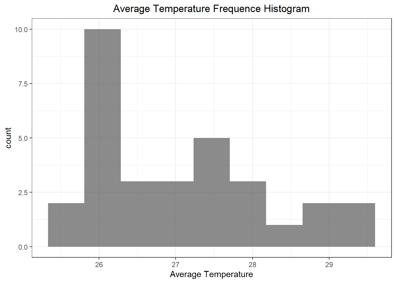
sensor$avg_temp## [1] 26.012653 25.879479 28.302872 25.967144 27.939340 25.517123 27.497169
## [8] 29.305905 25.850505 27.028029 7.879993 28.152182 28.858535 25.913236
## [15] 28.164899 26.645538 27.566751 27.299922 29.175229 26.378803 26.941640
## [22] 26.222689 26.964437 25.908585 26.734579 28.866217 26.185707 26.065050
## [29] 25.545073 27.256887 25.892882 27.382421sensor <- sensor %>% filter(avg_temp > 15)After these steps, size of data frame sensor is rapidly reduced from the original 497,912 to 32. The data frame now indicates average temperatures in the afternoon of 31 distinct sensor spots.
- Sensor data is already now.
- Merge sensor data with geographic location
- Then, convert the completed node data to spatial object format for plotting and more advanced spatial analytics.
nodes <- merge(sensor, nodes, by = c("node_id"))
coordinates(nodes) <- nodes[,c("lon", "lat")]
proj4string(nodes) <- CRS("+init=epsg:4326")
5.2.2 Descriptive Statistics
For the data is spatial, the most direct way is to plot a map.
tmap_mode("view")
tm_shape(nodes) + tm_dots()
From the map, we can get a general idea of the sensor position.
Chicago community area is the domain of the model. Recall the random process \(\{Z(s), s\in D\}\), which is the object of spatial analysis. The goal is to interpolate a temperature surface in \(D\). It is helpful to plot community area as well.
chiCA <- readOGR("../../Data","ChiComArea") # generated by the workshop## OGR data source with driver: ESRI Shapefile
## Source: "D:\Ryanna\RUC_courses\R_Y1_1\Geometrics\Data", layer: "ChiComArea"
## with 77 features
## It has 4 fields
## Integer64 fields read as strings: ComAreaIDtmap_mode("view")
tm_shape(chiCA) + tm_borders() +
tm_shape(nodes) + tm_dots(col="avg_temp",size=0.3, title="Average Temperature (C)") in Chicago community area (namely, \(D\)), temperature sensors are not clustered, which is good for modeling.
5.3 Model Fitting
5.3.1 Variogram
As an important parameter for spatial modeling, variogram has to be studied.
v <- variogram(nodes$avg_temp ~ 1, nodes)
plot(v)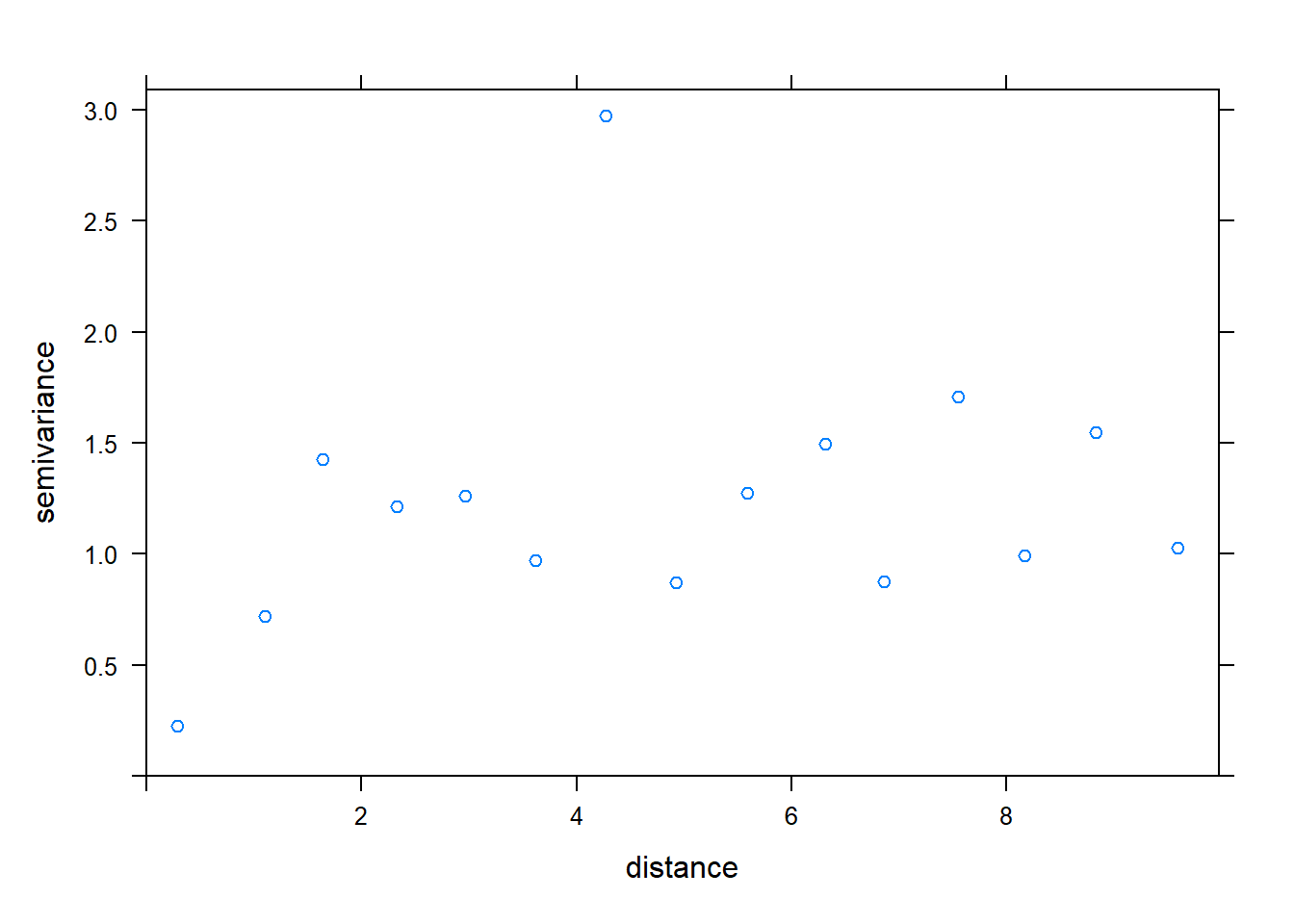
Observe the variogram, it seems spherical semivariogram (5.1), exponential variogram (5.2) can be suitable for the data.
Spherical Semivariogram
\begin{equation} ( ; )= \[\begin{cases}0, & \mathbf{h}=\mathbf{0}, \\ c_{0}+c_{s}\left\{(3 / 2)\left(\|\mathbf{h}\| / a_{s}\right)-(1 / 2)\left(\|\mathbf{h}\| / a_{s}\right)^{3}\right\}, & 0<\|\mathbf{h}\| \leq a_{s}, \\ c_{0}+c_{s}, & \|\mathbf{h}\| \geq a_{s},\end{cases}\]\(\theta=\left(c_{0}, c_{s}, a_{s}\right)^{\prime}\), \tag{5.1} \end{equaton} where \(c_{0} \geq 0, c_{s} \geq 0\), and \(a_{s} \geq 0\).
Exponential Variogram
\[\begin{equation} \gamma(\mathbf{h} ; \boldsymbol{\theta})= \begin{cases}0, & \mathbf{h}=\mathbf{0} \\ c_{0}+c_{e}\left\{1-\exp \left(-\|\mathbf{h}\| / a_{e}\right)\right\}, & \mathbf{h} \neq \mathbf{0}\end{cases}$ $\theta=\left(c_{0}, c_{e}, a_{e}\right)^{\prime}$, \tag{5.2} \end{equation}\] where \(c_{0} \geq 0, c_{e} \geq 0\), and $a_{e} .
v_fit_sph <- fit.variogram(v, model = vgm("Sph"))
plot(v, v_fit_sph)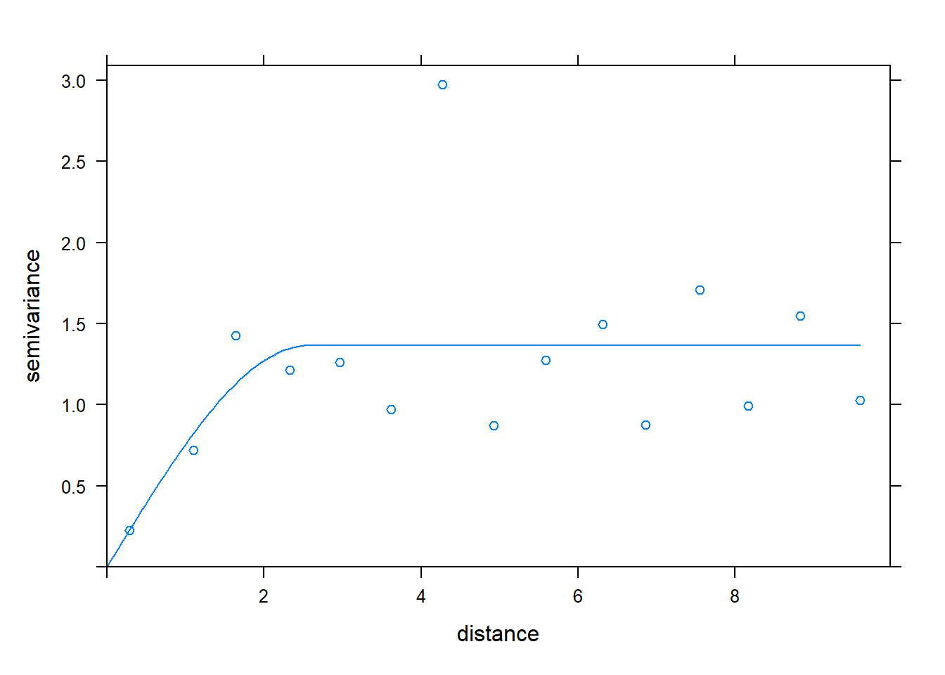
v_fit_exp <- fit.variogram(v, model = vgm("Exp"))
plot(v, v_fit_exp)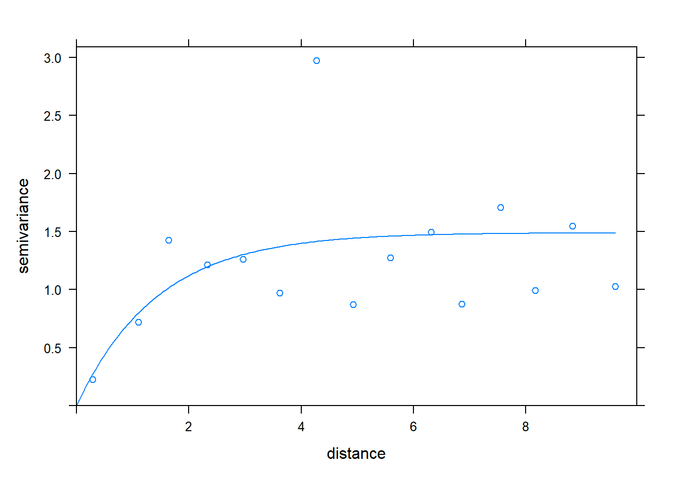
It is hard to choose the variogram model. We might as well adopt the relatively simpler exponential variogram for the following modeling.
5.3.2 Kriging Model
Gridding and projection should be performed before modeling kriging.
chi_grid <- pt2grid((chiCA), 200) # self-defined pt2grid for griding (omitted)
projection(chi_grid) <- CRS("+init=epsg:4326")
projection(nodes) <-  CRS("+init=epsg:4326")
projection(chiCA) <- CRS("+init=epsg:4326")
Then ordinary kriging model (illustrated in section 2.2) is fitted here.
kg <- krige(nodes$avg_temp ~ 1, nodes, chi_grid, model = v_fit_exp)## [using ordinary kriging]plot(kg)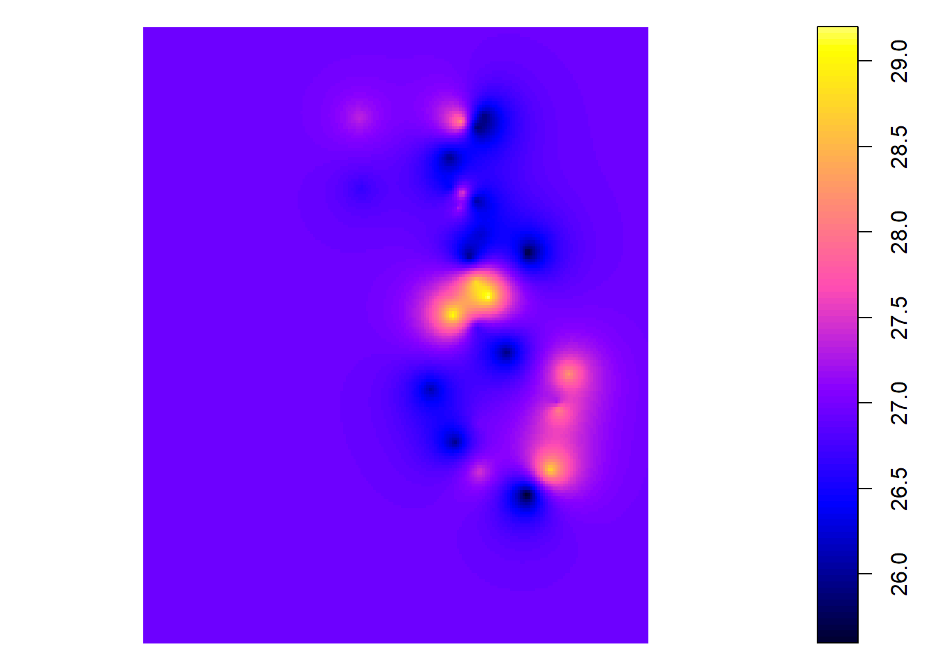
Clip the whole map to Chicago boundaries.
chi_kg <- kg[chiCA,]
plot(chi_kg)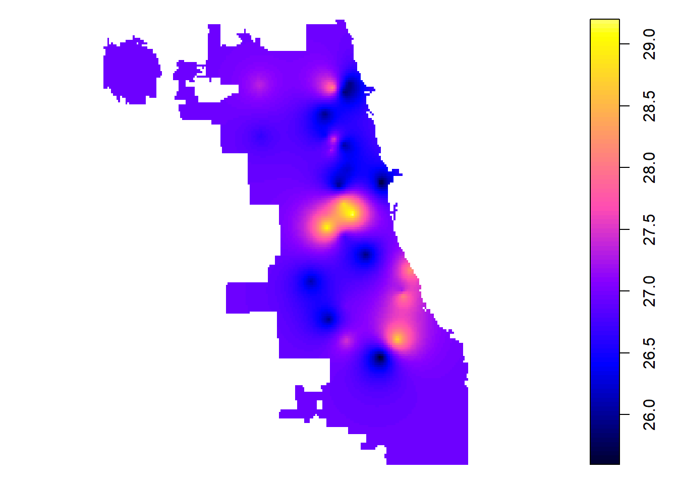
Combine the predicted temperature surface, community area and sensor information, the results can be plotted nicely as
tm_shape(chi_kg) +
  tm_raster("var1.pred", style = "jenks", title = "Temperature (C)", palette = "BuPu") + tm_shape(nodes) + tm_dots(size=0.01) +
  tm_layout(main.title = "Avg Afternoon Temperature August 25", main.title.size = 1.1) +
  tm_legend(position = c("left", "bottom"))
5.4 Animation
The analysis above interpolate average temperature of Augest 25, 2018. If we are interested in hourly average temperature, we can fit 24 models using the data. An animation of hourly change of temperature in Chicago is as below.
In practice, animation like this is informative and common. One main further modification of this animation is to uniform legend scale of different hour