Geostatistics Final Summary
2022-01-31
Chapter 1 Geostatistics
1.1 Targeted Problems
Spatial data is considered as a random process \(\{Z(s),s\in D\}\) in this part.
- \(D\): a is a fixed subset of \(\mathbb{R}^d\) with positive d-dimensional volume.
- \(s\): locations varies continuously throughout the region \(D\).
Set coalash dataset as an example (Figure 1.1). \(D\) is the region with values. and \(s\) indicates percent of coalash in this location. Many kinds of exploratory statistics can be applied here to test stationarity, local stationarity and so on.
Figure 1.1: Scatter Plot of CoalAsh Percent
The key idea in this chapter is to model the above random process \(\{Z(s),s\in D\}\) with values on known locations. Then inference of unknown locations can be made.
1.2 Spatial Data Example
1.2.1 Main Concepts
Variogram is the crucial parameter of geostatistics.
Intrinsic Stationarity
Based on the random process mentioned above, intrinsic stationarity is defined through first differences \[\begin{equation} \begin{aligned} &E\{Z(s+h) - Z(s)\} = 0,\\ &Var\{Z(s+h) - Z(s)\} = 2\gamma(h). \end{aligned} \tag{1.1} \end{equation}\]
Variogram
Variogram is \(2\gamma(h)\) in the definition of intrinsic stationarity.
1.2.2 Esitimation of Variogram
1.2.2.1 Estimator
The classical estimator of the variogram:
\[\begin{equation}
2 \hat{\gamma}(h) \equiv \frac{1}{|N(h)|} \sum_{N(h)}\left(Z\left(s_{i}\right)-Z\left(s_{j}\right)\right)^{2}
\tag{1.2}
\end{equation}\]
Estimator (1.2) is unbiased. However, it is badly affected by atypical observations due to square operation.
For an approximately symmetric distribution, there is a more robust approach to the estimation of the variogram by transforming the problem to location estimation. For a Gaussian process, we have:
\[\begin{equation} 2 \bar{\gamma}(\mathrm{h}) \equiv\left\{\frac{1}{|N(\mathrm{~h})|} \sum_{N(\mathrm{~h})}\left|Z\left(\mathrm{~s}_{i}\right)-Z\left(\mathrm{~s}_{j}\right)\right|^{1 / 2}\right\}^{4} /\left(0.457+\frac{0.494}{|N(\mathrm{~h})|}\right). \tag{1.3} \end{equation}\]
Estimator (1.3) is also unbiased.
1.2.2.2 Visualization
Variogram Cloud:
Cousin to estimator (1.2), variogram cloud is a useful diagnostic tool. Similarly, it can be badly affected by atypical observations. Variogram cloud in east-west direction of coalash data is shown in Figure 1.2
Here are steps to draw variogram cloud.
- Group points with \(y\) value;
- Calculate the classical estimator of the variogram \(\frac{1}{|N(h)|}\cdot \displaystyle\sum_{N(h)}{(z(s_i) - z(s_j))^2}\).
- \(N(h) = \{(s_i, s_j):\ s_i + he = s_j\}\)
- \(e\): the unit vector of east direction (positive x axis)
- Notice that y values of each pair \((s_i, s_j)\) are the same. But they may vary among pairs.
- Plot the corresponding boxplot.
- x axis: distance \(h\)
- y axis: the classical estimator of the variogram with parameter h, Units are \((\% coal ash)^2\)
Figure 1.2: Variogram Cloud in the East-West Direction
Square-Root-Differences Cloud:
The only different from variogram cloud: calculate the classical estimator of the variogram \(\frac{1}{|N(h)|}\cdot \displaystyle\sum_{N(h)}{|Z(s_i) - Z(s_j)|^\frac12}\).
Figure 1.3: Square-Root-Differences Cloud in the East-West Direction
Pocket Plot
The Pocket Plot tries to identify a localized area as being atypical with respect to a stationary mode. We plotting Pocket Plot 1.4 in the North-South Direction follows the steps as below:
- Get \(\{|N_{jk}|\}\) matrix (symmetric).
- Denote \(|N_{jk}|\) as the value of row \(j\) and column \(k\) of the matrix
- \(N_{jk} = \{(s_j, s_k):\ s_j \in row_j, s_k \in row_k, x_{s_j} = x_{s_k}\}\)
- \(|N_{jk}|\) means total pair number between row \(j\) and \(k\)
- Get \(\{Y_{jk}\}\) matrix (symmetric).
- For there are 23 distinct value in y axis, the matrix has the dim of \(23\times 23\)
- Denote \(Y_{jk}\) as the value of row \(j\) and column \(k\) of the matrix, we have \(Y_{jk} = \frac{1}{N_{jk}}\displaystyle\sum_{N_{jk}}|z(s_j) - z(s_k)|^{\frac12}\)
- Calculate \(Y_h\) vector.
- \(Y_h\) is the weighted mean of \(Y_{jk}\) where \(|j - k| = h\)
- Calculate \(P_{jk} = Y_{jk} - Y_h\)
- Plot the boxplot.
- x axis: index \(j\)
- y axis: \(P_{jk}\).
- There should be 23 points of each columns.
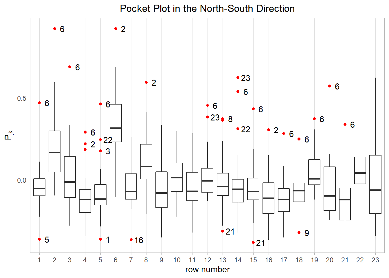
Figure 1.4: Pocket Plot in the North-South Direction
1.2.3 Decomposition
The goal is to deompose data into large- and small-scale variation.
Large-Scale Variation: The grand, column, and row effects.
Small-Scale Variation: The residual.
- Like ANOVA, \(F\) test within-rows and within-columns is first raised. However, it suffer from correlation among data points.
- Another additive decomposition follows the idea of \(data = all + row + column + residual\). Then for value of a location \((i,j)\) can be decomposed as \(Y_{ij} = Y_{..} + (Y_{i.}-Y_{..}) + (Y_{.j}-Y_{..}) + (Y_{ij}-Y_{i.}-Y_{.j}+Y_{..})\), where a subscripted dot (·) denotes averaging over that subscript. This can be settled by median polishing method.
Median Polishing
Successively sweeps medians out of rows, then columns, then rows, then columns, and so on, accumulating them in “row,” “column,” and “all” registers, and leaves behind the table of residuals.
1.3 Stationary Process
The concept of intrinsic stationarity has been introduced in section 1.2.1. Second-order (weak) stationarity is addressed in this section. It should be noticed that intrinsic stationarity is weaker than second-order stationarity.
Intrinsic Stationarity
Based on the random process mentioned above, intrinsic stationarity is defined through first differences \[\begin{equation} \begin{aligned} &E\{Z(s+h) - Z(s)\} = 0,\\ &Var\{Z(s+h) - Z(s)\} = 2\gamma(h). \end{aligned} \tag{1.1} \end{equation}\]
Second-Order (Weak) Stationarity
When the random process meets the following assuptions, the process is second-order (weak) stationary. \[\begin{equation} \begin{aligned} &E(Z(s)) = 0, \ \forall s \in D \\ &Cov(Z(s_i), Z(s_j)) = C(s_i - s_j), \ \forall s_i, s_j \in D \end{aligned} \tag{1.4} \end{equation}\]
Other important concepts related to stationary process as listed below.
- Covariogram: Function \(C(.)\) in (1.4).
- Isotropy: When \(C(s_i - s_j)\) only depends on \(\Vert s_i - s_j\Vert\) but not the direction of \(s_i - s_j\), then \(C(.)\) is isotropic.
- Anisotropy: Contrary to isotropy, when \(C(s_i - s_j)\) depends on both \(\Vert s_i - s_j\Vert\) and the direction of \(s_i - s_j\), then \(C(.)\) is anisotropic.
- Caused by underlying physical process evolving differentlly in space.
- The Euclidean space is not appropriate for measuring distance between locations.
- Ergodicity: The property which allows expectations over the \(\Omega \in \mathbb{R}^d}\) space to be estimated by spatial averages.
- Strong Stationarity: Strong stationarity refers to the property that the distribution of any finite sample of \(Z(.)\) is independent of locations (translation invariant).
1.3.1 Variogram & Covariogram
Recall section 1.2.1, variogram is defined as \(2\gamma(h) = Var(Z(s+h) - z(s)),\ \forall s, s+h\in D\). Some exploratory analysis of variogram has been seen in the example. Some related concepts are listed below.
- Semiv-variogram: \(\gamma(h) = \frac12 Var(Z(s+h) - z(s))\).
- Relative Variogram: Variogram of transformed data. Sometimes, simple transformations lead to intrinsic stationary processes.
- Nugget Effect: \(c_0\) is named as nugget effect, where \(c_0 = \lim_{h\to 0}\gamma(h)\).
- When \(h\to 0\), \(Var(Z(s+h) - Z(s))\to Var(0)\), which should be exactly 0. This implies that nuggest effect should be 0 if assumptions are all met.
- Causes of \(c_0 > 0\):
- Measurement error;
- Microscale variation.
- Estimation: Extrapolating the variogram estimates fro lags closest to zero. for practically, it is impossible to calculate variogram with scale less than \(\min \left\{\left\|s_{i}-s_{j}\right\|, 1 \leq i \leq j \leq n\right\}\).
- Still: The quantity \(C(0)\) is called still. \(C(0) - c_0\) is called the partial still.
Here are some other properties related to variogram and covariogram.
- Variogram is symmetric: \(\gamma(h) = \gamma(-h),\ \gamma(0) = 0\).
- Speed of increase: \(\lim _{|h| \rightarrow \infty} \frac{2 \gamma(h)}{|h|^{2}}=0\), which means that it is necessary for a variogram to increase slower than \(|h|^2\).
- Under stationarity, the covariance function \(C(h)\) is necessarily positive definite.
- Under intrinsic stationarity, variograms must be conditionally negative-definite.
1.3.2 Estimation of Variogram & Covariogram
1.3.2.1 Estimator of Variogram
Considering the definition of variogram, the most direct solution is moment estimator \[2 \hat{\gamma}(h) \equiv \frac{1}{|N(h)|} \sum_{N(h)}\left(Z\left(s_{i}\right)-Z\left(s_{j}\right)\right)^{2}\] where \(N(h) = \{(s_i, s_j): s_i - s_j = h\}\)
Generally speaking, the variogram estimator can be expressed as a quadratic form (1.5)
\[\begin{equation} 2\hat \gamma (h) = Z'A(h)Z \tag{1.5} \end{equation}\]
Denote \(Var(Z)=\Sigma\), then the means and variance of \(2\gamma(h)\) can be calculated as:
\[\begin{equation} \begin{aligned} E(2 \hat{\gamma}(h)) &=\operatorname{trace}(A(h) \Sigma) \\ \operatorname{var}(2 \hat{\gamma}(h)) &=2 \operatorname{trace}(A(h) \Sigma A(h) \Sigma) \end{aligned} \tag{1.6} \end{equation}\]
1.3.2.2 Estimator of Covariogram
For Covariogram, estimators are in line with basic ideas of variogram estimators. In the same way, the most direct thought of moment estimator is as Formula (??)
\[\begin{equation} \hat{C}(h) \equiv \frac{1}{|N(h)|} \displaystyle\sum_{N(b)}\left(Z\left(s_{i}\right)-\bar{Z}\right)\left(Z\left(s_{j}\right)-\bar{Z}\right) \end{equation}\]
where \(\bar{Z}=\sum_{i=1}^{n} Z\left(s_{i}\right) / n\).
1.3.3 Validity
Not all functions can be variograms or covariogram. There are some prerequisites ensuring validity of them.
1.3.3.1 Valid Variogram
- Under intrinsic stationarity, variogram must be conditionally negative definite, which means (1.7)
\[\begin{equation} \sum_{i, j} a_{i} a_{j} 2 \gamma\left(s_{i}-s_{j}\right) \leq 0$ for $\sum a_{i}=0 \tag{1.7} \end{equation}\]
- Continuous conditionally negative definite function corresponds to an intrinsically stationary stochastic process.
- Valid variogram forms a convex cone.
- Theorem 1.1 provides us with several ways to check variogram validity.
Theorem 1.1 If \(2 \gamma(.)\) is continuous on \(\mathbb{R}^{d}\) and \(\gamma(0)=0\), then the following are equivalent:
- \(2 \gamma(.)\) is conditionally negative definite;
- For all \(a>0\), \(\exp (-a \gamma(.))\) is positive definite.
- \(2 \gamma(h)=Q(h)+\int \frac{1-\cos \left(\omega^{\prime} h\right)}{\|\omega\|^{2}} G(d \omega)\), where \(Q(.) \geq 0\) is a quadratic form and \(G(.)\) is a positive, symmetric measure continuous at the origin that \(\int\left(1+\|\omega\|^{2}\right)^{-1} G(d \omega)<\infty\).
1.3.3.2 Valid Covariogram
- Under second-order stationarity, the covariance function \(C(h)\) is necessarily positive definite. That is, for any real numbers \(a_1,...,a_n\) and locations \(s_1,...,s_n\),
({i=1}^{n} a{i} Z(s_{i}))={i, j} a{i} a_{j} C(s_{i}-s_{j}) \tag{1.8} \end{equation}
- Spectral representation form
- Accoding to Theorem 1.2, a continuous function \(C(h)\) is positive-definite if and only if it has a spectral representation \(C(h)=\int \cos \left(\omega^{\prime} h\right) G(d \omega)\), where \(G\) is a positive bounded symmetric measure.
- Spectral density and distribution
- \(G/C(0)\) is the spectral distribution function
- If \(G(d \omega)=g(\omega) d \omega\), \(g/C(0)\) is the spectral density function.
- Accoding to Theorem 1.2, a continuous function \(C(h)\) is positive-definite if and only if it has a spectral representation \(C(h)=\int \cos \left(\omega^{\prime} h\right) G(d \omega)\), where \(G\) is a positive bounded symmetric measure.
Theorem 1.2 Theorem For any normalized continuous positive-definite function \(f\) on \(G\) (normalization here means that \(f\) is 1 at the unit of \(G\) ), there exists a unique probability measure \(\mu\) on \(\widehat{G}\) such that \[ f(g)=\int_{\widehat{G}} \xi(g) d \mu(\xi) \]
1.4 Variogram Model Fitting
Considering variogram validity prerequisites, variogram estimators presented in section 1.3.2.1 can not be used directly for spatial prediction. The key idea of variogram model fitting is to search for a valid variogram that is closest to the data.
When there are more than one valid model, probably from method illustrated from section 1.4.2 to 1.4.3.1, corss validation is an important tool for model checking.
1.4.1 EDA Check Before Model Fitting
- Check assumptions such as constant mean, constant marginal variance, stationarity, intrinsic stationarity;
- Check the Gaussian assumption;
- If the data is approximately normally distributed, modelling the first two moments are quite enough.
- If some evidence of non-Gaussianity is found, the variogram estimator defined in section 1.3.2.1 is still valid, because they can be viewed as moment estimators which are independent of Gaussian assumption.
- Isolate suspicious observations for further study;
- Choose a appropriate parametric variogram model.
From now on, we consider
1.4.2 Maximum Likelihood Estimator
- Assumptions:
- Suppose the data is generated from a stationary Gaussian process with a parametric variogram model \(P=\{2 \gamma: 2 \gamma(h)=2 \gamma(h ; \theta) ; \theta \in \Theta\}\). Then the goal is to estimate \(\theta\).
- Suppose we also observed some covariates \(X_1,...,X_n\) which are linearly related to \(Z\).
- Model: \(Z=\left(Z\left(s_{1}\right), \ldots, Z\left(s_{n}\right)\right) \sim N(X \beta, \Sigma(\theta))\) where \(\Sigma(\theta)=\left(\operatorname{cov}\left(Z\left(s_{i}\right), Z\left(s_{j}\right)\right)\right)\).
- Goal: find parameter estimation \((\hat \beta, \hat \theta)\) to minimize loglikelihood function (1.9).
- Where there is no spatial correlation, this amounts to a simple linear regression model. The solution is \(\Sigma(\theta)=\sigma^{2} I\) and \(\theta=\sigma^{2}.\)
- General solution: \(\hat{\sigma}^{2}=\sum\left(Z\left(s_{i}\right)-X_{i} \hat{\beta}\right)^{2} / n\)
- \(\hat{\sigma}^{2}\) is biased.
- For \(E\left(\hat{\sigma}^{2}\right)=(n-q) / n \sigma^{2}\), the larger \(q\) is, the more biased the estimator gets.
\[\begin{equation} L(\beta, \theta)=\frac{n}{2} \log (2 \pi)+\frac{1}{2} \log |\Sigma(\theta)|+\frac{1}{2}(Z-X \beta)^{\prime} \Sigma(\theta)^{-1}(Z-X \beta) \tag{1.9} \end{equation}\]
- Improvements: To de-bias \(\hat \theta\), which is \(\hat{\sigma}^{2}\) is out case, restricted maximum likelihood estimator (EMLE) is raised.
- Estimator form: \(\hat{\theta}=\int_{\beta} \exp (-L(\beta, \theta))(d \beta)\)
Once variogram is estimated, then covariogram can be easily get by \(2\gamma(h) = 2(C(0) - C(h))\)
1.4.3 MINQ Estimation
Applicable Situation: the variance matrix of the data is linear in its parameters, i.e. \(\Sigma(\theta)=\theta_{1} \Sigma_{1}+\ldots, \theta_{m} \Sigma_{m}\). The MINQ approach is particularly appropriate for a variance components model.
1.4.3.1 Least Squares Esimator
The main idea of Least Squares Esimator (LSE) is the same as least square regression. The goal function to minimize is the square error.
\[\begin{equation} \sum_{j=1}^{K}\left\{2 \gamma^{\#}(h(j) e)-2 \gamma(h(j) e ; \theta)\right\}^{2} \tag{1.10} \end{equation}\]
If we not \(2 \boldsymbol{\gamma}^{\#}=\left(2 \gamma^{\#}(h(1)), \ldots, 2 \gamma^{\#}(h(K))\right)\) with covariance matrix \(\operatorname{var}\left(2 \boldsymbol{\gamma}^{\#}\right)=V\), the goal to minimize is tranformed into
\[\begin{equation} \left(2 \boldsymbol{\gamma}^{\#}-2 \boldsymbol{\gamma}(\theta)\right)^{\prime} V^{-1}\left(2 \boldsymbol{\gamma}^{\#}-2 \boldsymbol{\gamma}(\theta)\right) \tag{1.11} \end{equation}\]
- Notice that although a direction vector \(e\) is included in formula (1.10), multiple directions could also be accounted for by adding the appropriate squared differences.
- Drawbacks: The least squares estimator takes no cognizance of the distributional variation and covariation of the generic estimator.
- Improvement:
- Weighted Least Squares (WLS): Replace \(V\) by a diagonal matrix \(\left.\Delta=\operatorname{diag}\left(\operatorname{var}\left(2 \gamma^{\#}(h(1))\right), \ldots, 2 \gamma^{\#}(h(K))\right)\right)\).
- Generalized Least Squares (GLS): use just the (asymptotic) second-order structure of the variogram estimator and does not make assumptions about the whole distribution of the data. When there is little knowledge of the true model, GLS is a good startingg choice.