6 Exercise 4 - Power and Weight

In an experiment conducted by the GU physiology department, a sample of volunteers had their power output measured (in watts) while they ran up stairs as fast as possible under different test conditions. Their gender was noted and their weight and leg length measurements recorded. The data are available from the csv file phys1.csv . To open this data file in RStudio type:

phys <- read.csv("phys1.csv")

This will assign the data to the object phys. This worksheet contains six columns, described as follows:

             C1: Gender
             C2: Weight (kgs)
             C3: Leg Length (metres)
             C4: Power1: Power output in the stair test
             C5: Power2: Power output in a test with a ramp on the stairs
             C6: Power3: Power output with ramp on the stairs and a fixed stride length

You can view these names using names(phys)
To view a spreadsheet of the data, use fix(phys)
The spreadsheet can also be viewed by clicking on the phys object in the Workspace (top right of the screen).

6.1 Exploratory analysis

(a) i. Create a simple scatterplot of Power1 vs Weight

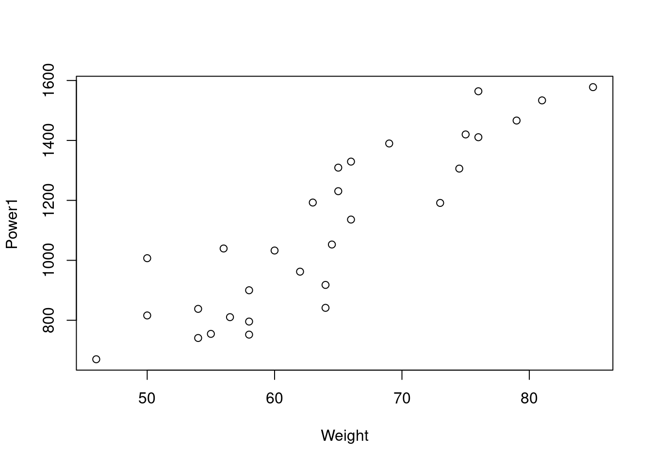
phys <- read.csv("phys.csv")
plot(Power1 ~ Weight, data = phys)

ii. Adjust the labelling on your plot to look like the following:

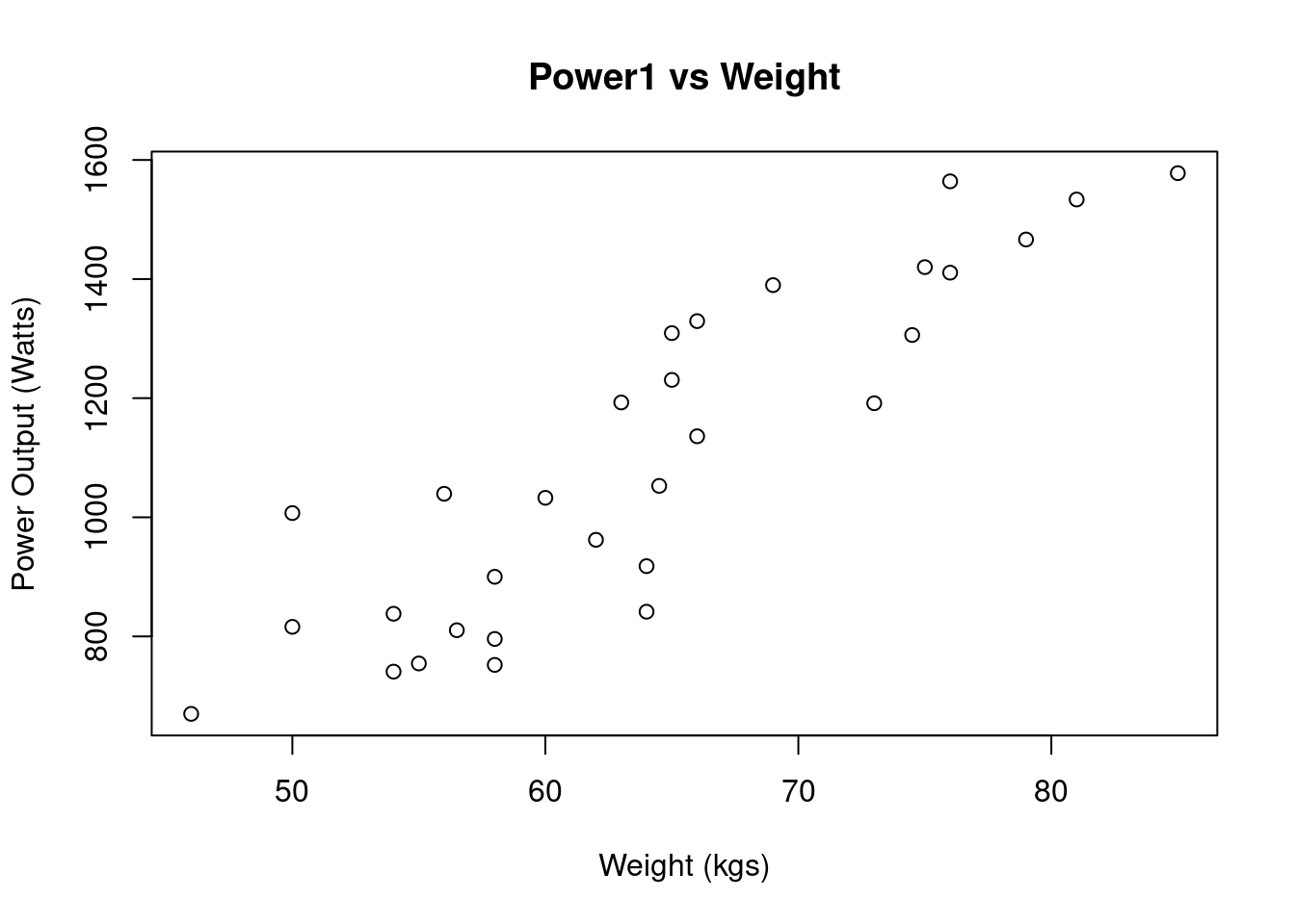
Labels and titles can be added as parameters in your plot() code. For help on the possible paramters you can run the code help(plot) or press f1 on your keyboard when your curser is on the plot code.

phys <- read.csv("phys.csv")
plot(Power1 ~ Weight, data = phys, main="Power1 vs Weight", xlab = "Weight (kgs)",
ylab = "Power Output (Watts)")

iii. Adjust your code again to change your plot to look like the following (you should set the size of the points to 1.5):

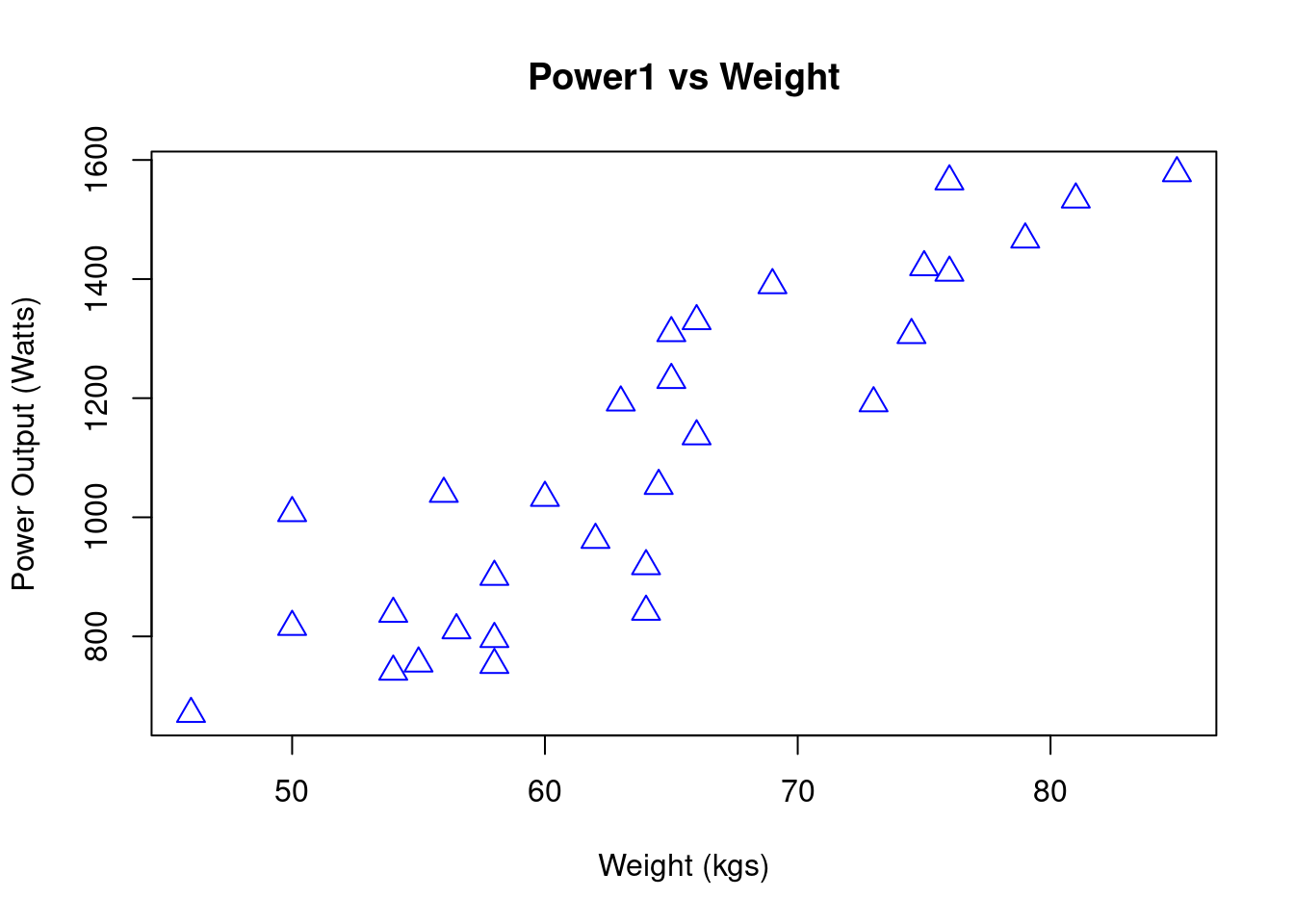
Colours and plot graphics can be changed using parameters in your plot() code. For help on the possible paramters you can run the code help(graphical parameters) or press f1 on your keyboard when your curser is on the plot code.

phys <- read.csv("phys.csv")
plot(Power1 ~ Weight, data = phys, main="Power1 vs Weight", xlab = "Weight (kgs)",
ylab = "Power Output (Watts)", pch = 2, cex = 1.5, col = "blue")

iv. What can we say about the relationship between Power Output and Weight?

The trend is and

6.2 More advanced scatterplots

We may want to look at the the possibility that any relationship between Power1 and Weight might be different for males and females. So, we now label the plot according to the gender of the subjects.

(b) i. Define a new group Gender1 as a character:

Gender1 <- as.character(phys$Gender)

Note that here, the $ sign extracts the variable Gender from the dataframe phys.

This will now allow the plot function to display a different character for each category in 'Gender' In this study this is Male and Female.

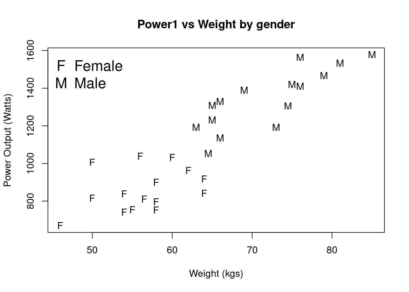
ii. Incorporate the Gender1 code into your scatter plot to label the points by gender:

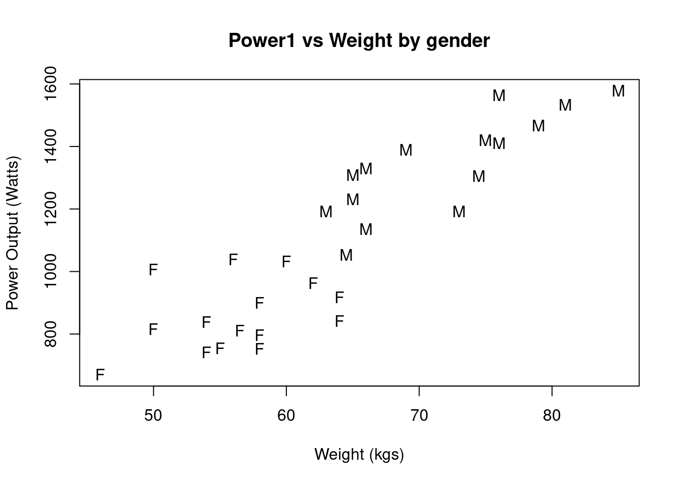
plot(Power1 ~ Weight, data = phys, xlab = "Weight (kgs)",
ylab = "Power Output (Watts)", main= "Power1 vs Weight by gender", pch = Gender1)

iii. Complete this plot by adding a legend:

For help on legends help(legends) or press f1 on your keyboard when your curser is on the code 'legend'.

plot(Power1 ~ Weight, data = phys, xlab = "Weight (kgs)",
ylab = "Power Output (Watts)", main= "Power1 vs Weight by gender", pch = Gender1)
legend("topleft", legend = c("Female", "Male"),
pch = c("F", "M"), bty = "n", cex = 1.5)