7 Tutorial 7: Data Analysis
After working through Tutorial 7, you’ll…
- understand how to calculate basic descriptive statistics in R.
- understand how to do run a linear regression in R.
Data
We again load the data frame data_combined which we created in Tutorial 5: Matching survey data & data donations.
You will find this R environment via Moodle under the folder “Data for R” (“tutorial6.RData”).
Use the load() command to load it to your working environment.
Let’s remember what this data contained:
- Our automated content analysis of YouTube search queries:
- Anonymous ID for each participant: external_submission_ID
- Share of news-related searches: share
- Our survey data:
- Anonymous ID for each participant: ID
- Sociodemographic characteristics: Age, Gender, Education
- Political Interest: PI1, PI2, PI3, PI4, PI5
- Social Media Use: Use_FB, Use_TWI, Use_INST, Use_YOU, Use_TELE, Use_WHATS
- Trust in News Media: Trust
We include some preparation for the survey data. These are all steps we already learned about in Tutorial 6: Preparing survey data:
- We create a dichotomous variable University indicating whether participants have a university degree (1) or not (0)
- We create a mean index of Political Interest consisting of the variables PI1, PI2, PI3, PI4, and PI5.
data_combined <- data_combined %>%

  ###Create new variable "University ##
  mutate(University = Education,
         University = replace(University,
                              Education != "University Degree",
                              "No University Degree")) %>%

  ##Create new mean index "Political Interest"
    add_index(PoliticalInterest,
            starts_with("PI"),
            type = "mean",
            cast.numeric = T)
This is how our data set looks like:
## # A tibble: 1 × 19
##   external_submission_id share   Age Gender Education   PI1   PI2   PI3   PI4   PI5 Use_FB Use_TWI Use_INST Use_YOU
##                    <int> <dbl> <int> <chr>  <chr>     <int> <int> <int> <int> <int>  <int>   <int>    <int>   <int>
## 1                   3861     0    18 Male   A-levels      3     1     2     2     2      1       2        4       3
## # ℹ 5 more variables: Use_TELE <int>, Use_WHATS <int>, Trust <int>, University <chr>, PoliticalInterest <dbl>
7.1 Descriptive statistics
Let’s start with simple descriptive summary statistics on our data.
7.1.1 Counts
For many variables - especially those with nominal or ordinal scale levels - you may want to count values. For instance, you may want to know how many participants in our data set have a university degree.
You can get this information using count() from the dplyr package.
In short, we summarize how many observations contain either 0, i.e., No University Degree, or 1, i.e., University Degree.
## # A tibble: 2 × 2
##   University               n
##   <chr>                <int>
## 1 No University Degree    38
## 2 University Degree       45
7.1.2 Percentages
Sometimes, it may be more helpful to not know how often a specific value occurs in absolute, but in relative terms, for example in percentages. To calculate this, we use an additional command called prop.table() to create a new variable called perc, which is merely the relative occurrence with which participants have a university degree.
## # A tibble: 2 × 3
##   University               n  perc
##   <chr>                <int> <dbl>
## 1 No University Degree    38  45.8
## 2 University Degree       45  54.2
7.1.3 Mean, standard deviation, etc.
For variables with metric scale levels, you may be interested in other types of summary statistics.
Remember our mean index on political interest PoliticalInterest which ranges from low interest in politics (1) to strong interest in politics (5).
We summarize the mean value participantes scored on PoliticalInterest by creating a new variable summarizing the value of PoliticalInterest via summarize() and mean():
## # A tibble: 1 × 1
##    mean
##   <dbl>
## 1  3.59
Or you could instead get the median with median() (for instance if you have extreme values skewing the distribution of the variable, in case of which “average” values may be better represented by the median):
## # A tibble: 1 × 1
##   median
##    <dbl>
## 1    3.8
Another useful value is the standard deviation via sd():
## # A tibble: 1 × 1
##      sd
##   <dbl>
## 1 0.975
Lastly, you already know how to round numeric data to a number of decimals to your choice (for instance to report them in a seminar paper):
## # A tibble: 1 × 1
##    mean
##   <dbl>
## 1   3.6
7.1.4 Summary statistics across groups
In some cases, you may also wish to get descriptive data for groups within our data. For instance, we may want to know how the frequency of news-related search varies across different values of Gender.
Using the dplyr package, we use the following code to get this information:
- We define the object to which functions should be applied: data_combined
- We group our data alongside the variable Gender
- We calculate the mean of news-related searches, here saved via share, across values of Gender
## # A tibble: 3 × 2
##   Gender  mean
##   <chr>  <dbl>
## 1 Female 0.475
## 2 Male   0.876
## 3 Other  0
Results indicate that male participants may slightly more often use YouTube for news-related searches - but we will have to use multivariate statistics to see whether translates to a consistent correlation between share and Gender.
Let’s do this next!
7.2 Linear regression
R offers a lot of options for doing inferential tests. Here, we will focus on a simple linear regression model:
We test whether the frequency with which participants use YouTube for news-related searches - variable share - correlates with sociodemographic characteristics - Age, Gender, and University - as well as their political interest - PoliticalInterest.
In R, we can run a linear regression using the lm() command.
Here, we have to specify two arguments:
- formula: this argument defines how we want to model our data. Here, we use share as the dependent variable and Age, Gender, University, and PoliticalInterest as independent variables.
- data: this argument defines where the function can find the data set based on the model will be run.
Let’s try this and save the result in a new object called model:
model <- lm(formula = "share ~ Age + Gender + University + PoliticalInterest",
            data = data_combined)
To visualize results, I recommend using the tab_model() command from the sjPlot package. It nicely visualizes all relevant results in a table.
Here, we also print standardized beta coefficients via the argument show.std7. Standardized coefficents are often easier to interpret, especially if we want to compare the influence of different independent variables.
The result looks like this:
| share | |||||
|---|---|---|---|---|---|
| Predictors | Estimates | std. Beta | CI | standardized CI | p |
| (Intercept) | -0.34 | -0.22 | -1.72 – 1.05 | -0.61 – 0.18 | 0.628 |
| Age | 0.01 | 0.07 | -0.01 – 0.02 | -0.18 – 0.32 | 0.566 |
| Gender [Male] | 0.56 | 0.44 | -0.08 – 1.19 | -0.06 – 0.94 | 0.084 |
| Gender [Other] | -0.38 | -0.30 | -2.25 – 1.48 | -1.78 – 1.17 | 0.684 |
|
University [University Degree] |
0.05 | 0.04 | -0.53 – 0.62 | -0.42 – 0.49 | 0.865 |
| PoliticalInterest | 0.13 | 0.10 | -0.18 – 0.45 | -0.14 – 0.34 | 0.393 |
| Observations | 83 | ||||
| R2 / R2 adjusted | 0.050 / -0.012 | ||||
How can we interpret our findings?
7.2.1 Model fit
a. Number of observations: Observations tell us that our data set contains N = 83 observations. That is a fairly low number which is partly due to people not wanting to donate their data. We have to keep this in mind, as running a regression with 83 cases is borderline okay, at best. But for the purpose of this seminar, discussing this critically in the discussion of your seminar paper is fine.
b. Explained Variance: Based on \(R^{2}\) = .05 and \(R^{2} adjusted\) = -.012, we see that our independent variables explain little to no variance in our dependent variable share. Overall, our explained variance is close to zero, indicating that sociodemographic variables and political interest bear little to no correlation with the degree to which participants use YouTube to search for news.
7.2.2 Interpreting Estimates
a. Age: Related to the variable Age, we see that participants’ age is not consistently correlated with using YouTube to search for news.
The standardized beta coefficient amounts to \(\beta_{age}\) = .07. The standardized confidence interval includes zero with \(CI_{lower}\) = -.18 and \(CI_{upper}\) = .32. Also, the p-value indicates a non-significant relationship with p = .566. In short, we would report this result as: There is no significant correlation between participants’ age and using YouTube to search for news, with \(\beta_{age}\) = .07, p = .566 [\(CI_{lower}\) = -.18; \(CI_{upper}\) = .32].
b. Gender: Related to the variable Gender, we see that participants’ gender is not consistently correlated with using YouTube to search for news.
This is true both for male participants compared to female participants, with \(\beta_{male}\) = .44, p = .084 [\(CI_{lower}\) = -.06; \(CI_{upper}\) = .94] and for participant identifying as other compared to female participants, with \(\beta_{other}\) = -.3, p = .684 [\(CI_{lower}\) = -1.78; \(CI_{upper}\) = 1.17].
c. University: Related to the variable University, we see that there is no significant correlation between participants’ education and using YouTube to search for news, with \(\beta_{university}\) = .04, p = .865 [\(CI_{lower}\) = -.42; \(CI_{upper}\) = .49].
d. Political Interest: Related to the variable PoliticalInterest, we see that here is no significant correlation between participants’ political interest and using YouTube to search for news, with \(\beta_{political interest}\) = .1, p = .393 [\(CI_{lower}\) = -.14; \(CI_{upper}\) = .34].
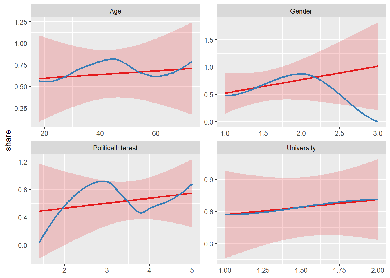
7.2.3 Checking regression slopes
If you want visualized regression slopes (for instance to check for non-linear relationships), you can also use the plot_model() command:
7.2.4 Model Assumptions
When checking your result, you should always bear in mind that you need to check model assumptions.
For linear regression models these assumptions include8…
- No Multicollinearity: Is there a strong correlation between independent variables? Variance Inflation Factors (VIF) above 5 or even 10 indicate multicollinearity. If this is the case, you could remove highly correlated independent variables.
- Normality of residuals/no outliers: Are error terms normally distributed/does the model not suffer from influential outliers? If this is the case, you could try either removing influential observations or using another model specification (e.g., log-transformation of variables; non-linear model)
- Homoscedastictiy: Is error spread constantly across values of the dependent variable? If there is a discernible pattern in the variance of residuals (e.g., a funnel distribution), this indicates heteroscedasticity. If this is the case, you could try another model specification (e.g., log-transformation of variables; non-linear model).
You can check assumptions via the plot_model() command:
## [[1]]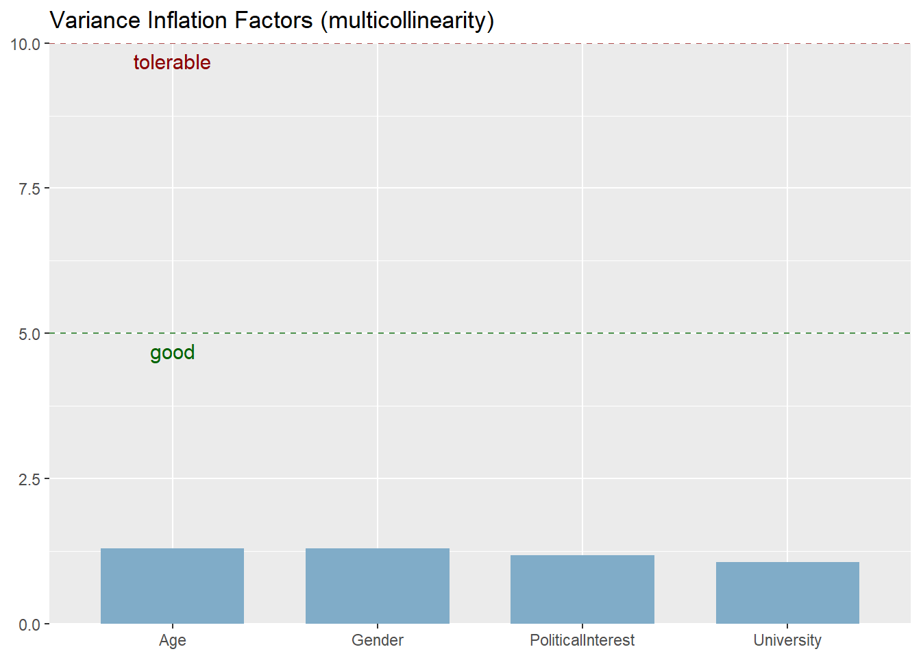
##
## [[2]]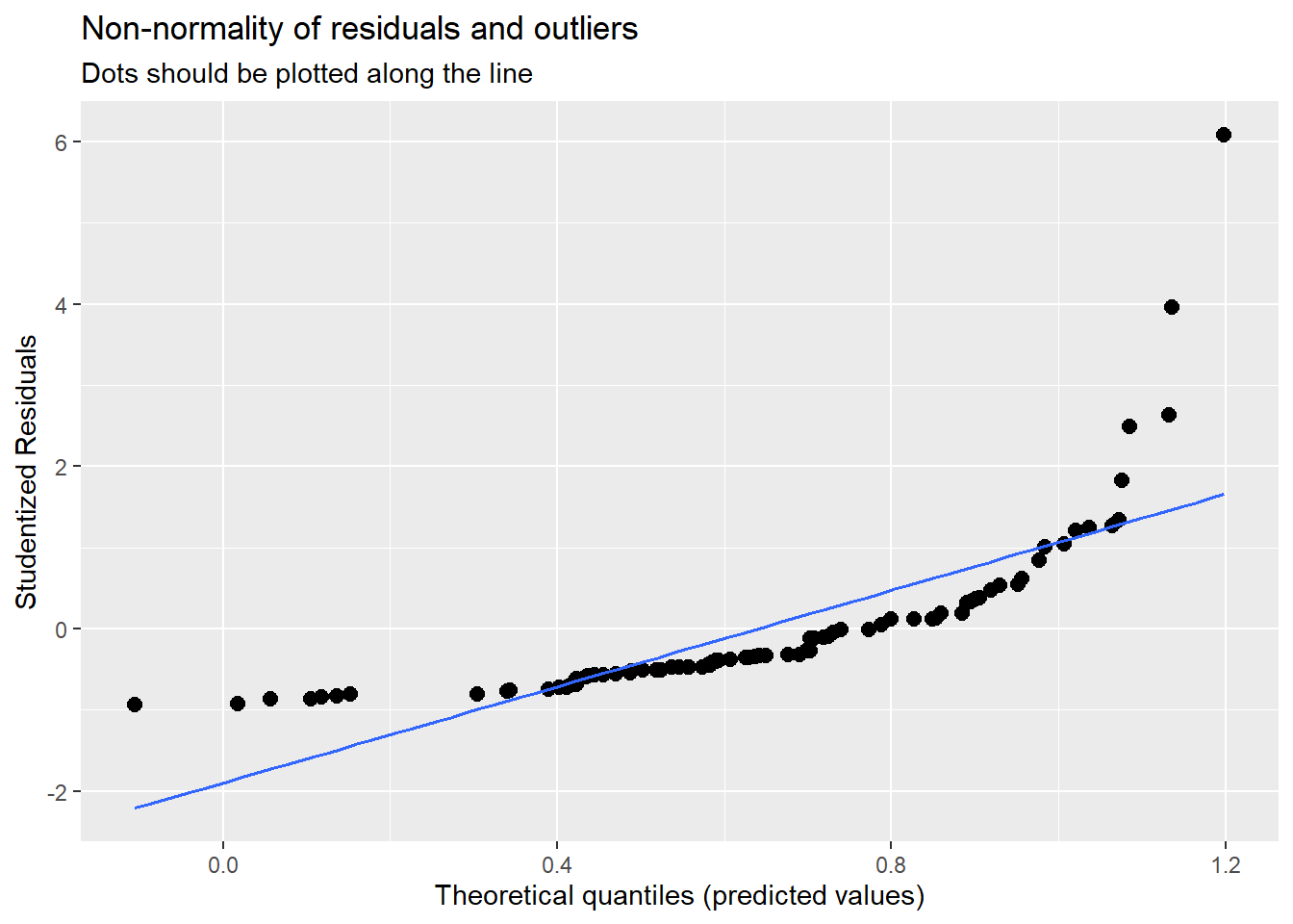
##
## [[3]]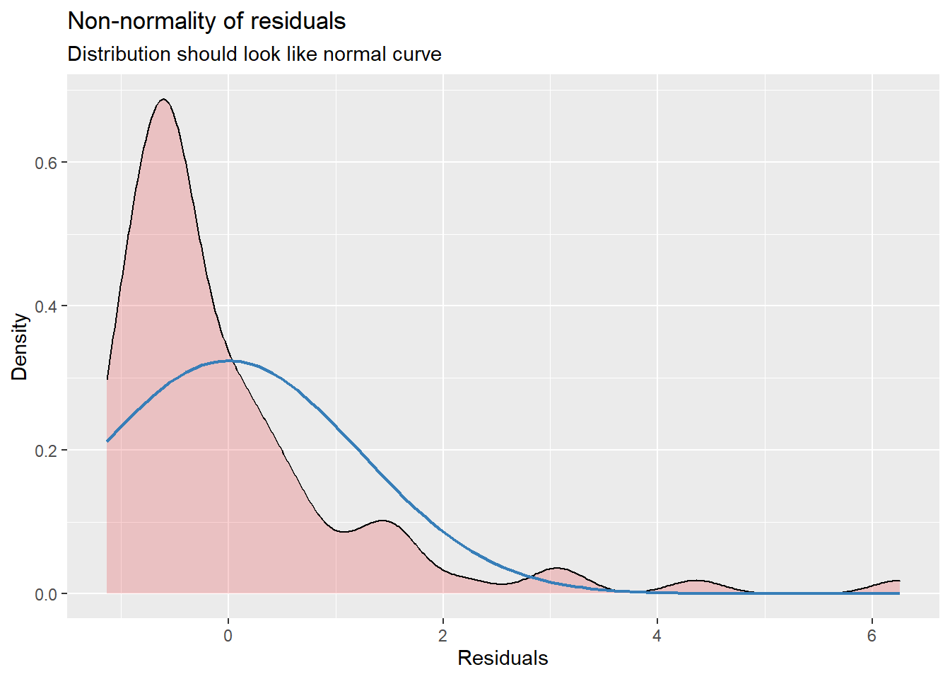
##
## [[4]]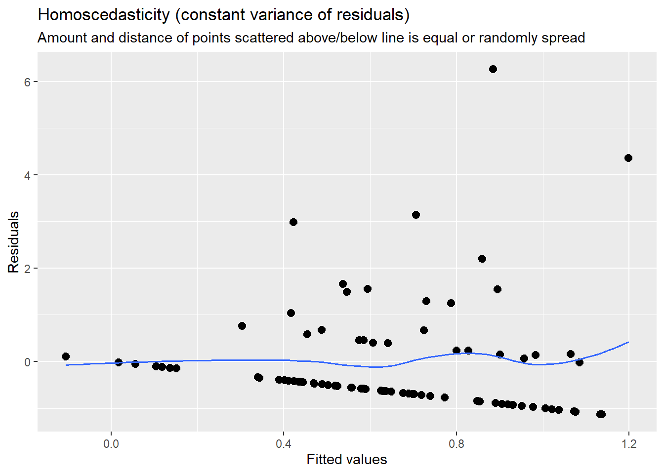
Overall, the assumption check that model assumptions, especially related to the normality of residuals and homoscedasticity, are at least partly violated, indicating poor model fit.
In turn, we could try whether other model specifications may make more sense - or whether it is simply the case that our independent variables bear not consistent correlation with the dependent variable.
7.3 More tutorials on this
You still have questions? The following tutorials & papers can help you with that:
7.4 Take Aways
Commands:
- Descriptive statistics: count(), prop.table(), mean(), median(), sd(), summarize()
- Linear regression: lm(), tab_model()
- Testing model assumptions: plot_model()
7.5 Test your knowledge
You’ve worked through all the material of Tutorial 7? Let’s see it - the following tasks will test your knowledge.
7.5.1 Task 7.1
Writing the corresponding R code, run another regression model where you include Age, Gender, University, PoliticalInterest, Trust, and Use_You as independent variables.
7.5.2 Task 7.2
Writing the corresponding R code, check and report whether underlying model assumptions are fulfilled.
7.5.3 Task 7.3
Based on the model you ran in Task 7.1: Does participants’ general use of YouTube, Use_You, correlate with the degree to which they use Youtube for news-related searches? Discuss findings based on the regression output.
Let’s keep going: with Tutorial 8: Visualizing results